Genetic Algorithms (M3.1)

 

Biological Background, Schema, Theorem, GA Operators: Crossover, Mutation and Its Types-GA Algorithm, Variations Of GA: Adaptive GA and Real Coded GA

Simulated Annealing (M2.2)

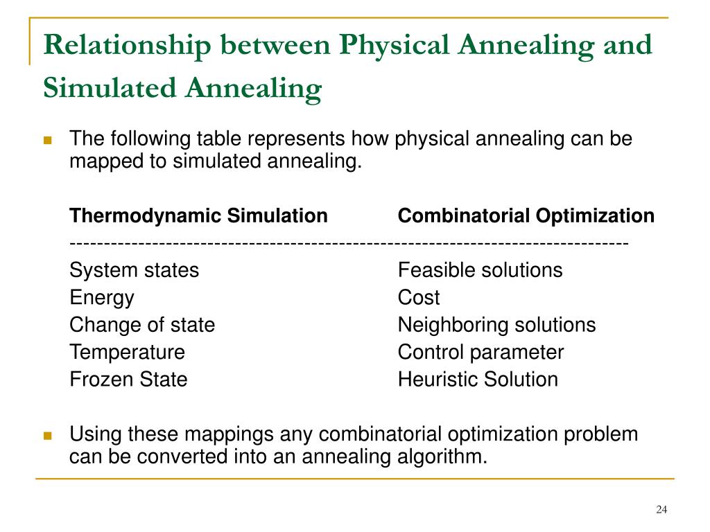
• SA algorithm is one of the most preferred heuristic methods for solving optimization problems. 

• It is a probabilistic technique which is an effective and general form of optimization. 

• It is useful in finding global optima of a given function when there is lot of local optima. 

• “Annealing” (heat (metal or glass) and allow it to cool slowly, in order to remove internal stresses and toughen it) refers to an analogy with thermodynamics, specifically with the way that metals cool and anneal. 

• Simulated annealing uses the objective function of an optimization problem instead of the energy of a material.

Simulated annealing is based on metallurgical practices by which a material is heated to a high temperature and cooled. At high temperatures, atoms may shift unpredictably, often eliminating impurities as the material cools into a pure crystal. This is replicated via the simulated annealing optimization algorithm, with energy state corresponding to current solution.

Physical Annealing:

• Simulated Annealing (SA) mimics the Physical Annealing process but is used for optimizing parameters in a model. 
• The Simulated Annealing algorithm is based upon Physical Annealing in real life. 
• Physical Annealing is the process of heating up a material until it reaches an annealing temperature and then it will be cooled down slowly in order to change the material to a desired structure. 
• When the material is hot, the molecular structure is weaker and is more susceptible to change. 
• When the material cools down, the molecular structure is harder and is less susceptible to change.

Another important part of this analogy is the following equation from Thermal Dynamics:

This equation calculates the probability that the Energy Magnitude will increase. We can calculate this value given some Energy Magnitude and some temperature t along with the Boltzmann constant k.

 

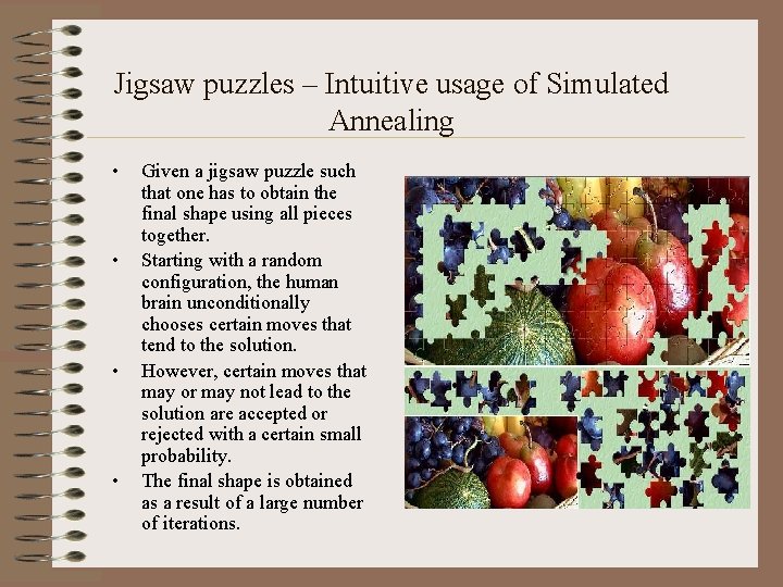
Implementation of SA is surprisingly simple.  The algorithm is basically hill-climbing except instead of picking the best move, it picks a random move.  If the selected move improves the solution, then it is always accepted.  Otherwise, the algorithm makes the move anyway with some probability less than 1.  The probability decreases exponentially with the “badness” of the move, which is the amount ΔE by which the solution is worsened (i.e., energy is increased.)

Acceptance Criteria

The law of thermodynamics state that at temperature, T, the probability of

an increase in energy of magnitude, ΔE, is given by

P(ΔE) = e−ΔE/kT

where k is a constant that relates temperature to energy known as Boltzmann’s constant.

At higher values of T, uphill moves are more likely to occur.  As T tends to zero, they become more and more unlikely, until the algorithm behaves more or less like hill-climbing.  

In a typical SA optimization, T starts high and is gradually decreased according to an “annealing schedule”. 

A certain number of iterations are carried out at each temperature and then the temperature is decreased. This is repeated until the system freezes into a steady state.

This equation is directly used in simulated annealing, although it is usual to drop the Boltzmann constant as this was only introduced into the equation to cope with different materials. Therefore, the probability of accepting a worse state is given by the equation

P = e−ΔE/T > r

where, ΔE= the change in the evaluation function

T= the current temperature

r= a random number between 0 and 1

The probability of accepting a worse move is a function of both the temperature of the system and of the change in the cost function.

As the temperature of the system decreases the probability of accepting a worse move is decreased. This is the same as gradually moving to a frozen state in physical annealing.

Also if the temperature is zero then only better moves will be accepted which effectively makes simulated annealing act like hill climbing.

Simulated annealing is typically used in discrete, but very large, configuration spaces, such as the set of possible orders of cities in the Traveling Salesman problem and in VLSI routing. It has a broad range of application that is still being explored.

Annealing schedule

The mapping of time to temperature and how fast the temperature decreases is called the Annealing Schedule. 

The algorithm starts initially with ${\displaystyle T}$ set to a high value (or infinity), and then it is decreased at each step following some annealing schedule—which may be specified by the user, but must end with ${\displaystyle T=0}$ towards the end of the allotted time budget. In this way, the system is expected to wander initially towards a broad region of the search space containing good solutions, ignoring small features of the energy function; then drift towards low-energy regions that become narrower and narrower; and finally move downhill according to the steepest descent heuristic.

For any given finite problem, the probability that the simulated annealing algorithm terminates with a global optimal solution approaches 1 as the annealing schedule is extended. This theoretical result, however, is not particularly helpful, since the time required to ensure a significant probability of success will usually exceed the time required for a complete search of the solution space.

Pseudocode

The following pseudocode presents the simulated annealing heuristic as described above. It starts from a state s₀ and continues until a maximum of k_max steps have been taken. In the process, the call neighbour(s) should generate a randomly chosen neighbour of a given state s; the call random(0, 1) should pick and return a value in the range [0, 1], uniformly at random. The annealing schedule is defined by the call temperature(r), which should yield the temperature to use, given the fraction r of the time budget that has been expended so far. 

• Let s = s₀
• For k = 0 through k_max (exclusive):
  • T ← temperature( (k+1)/k_max )
  • Pick a random neighbour, s_new ← neighbour(s)
  • If P(E(s), E(s_new), T) ≥ random(0, 1):
    • s ← s_new
• Output: the final state s
  

First, generate a random solution

We can do this however we want. The main point is that it's random - it doesn't need to be your best guess at the optimal solution.

Calculate its cost using some cost function you've defined

This, too, is entirely up to you. Depending on your problem, it might be as simple as counting the total number of miles the traveling salesman's traveled. Or it might be an incredibly complex melding of multiple factors. Calculating the cost of each solution is often the most expensive part of the
algorithm, so it pays to keep it simple.

Generate a random neighboring solution

"Neighboring" means there's only one thing that differs between the old solution and the new solution. Effectively, you switch two elements of your solution and recalculate the cost. The main requirement is that it be done randomly.

Calculate the new solution's cost

Use the same cost function as above. You can see why it needs to perform well - it gets called with each iteration of the algorithm.

If cnew < cold: move to the new solution

If the new solution has a smaller cost than the old solution, the new one is better. This makes the algorithm happy - it's getting closer to an optimum. It will "move" to that new solution, saving it as the base for its next iteration.

If cnew > cold: maybe move to the new solution

This is where things get interesting. Most of the time, the algorithm will avoid moving to a worse solution. If it did that all of the time, though, it would get caught at local maxima. To avoid that problem, it sometimes elects to keep the worse solution. To decide, the algorithm calculates something called the 'acceptance probability' and then compares it to a random number.

#Selecting the parameters

In order to apply the simulated annealing method to a specific problem, one must specify the following parameters: 

• state space, 
• energy (goal) function E(), 
• candidate generator procedure neighbour(), 
• acceptance probability function P(), 
• annealing schedule temperature() 
• initial temperature <init temp>. 

These choices can have a significant impact on the method's effectiveness. Unfortunately, there are no choices of these parameters that will be good for all problems, and there is no general way to find the best choices for a given problem.  

Known issues

Parameter setting is the significant part to the algorithm

SA works fine only if the parameters set correctly

Too low temperature: get stuck on a local minimum

Too high temperature: the optimum will be passed several times

Too large neighborhood: high complexity
 

Sometimes it is better to move back to a solution that was significantly better rather than always moving from the current state. This process is called restarting of simulated annealing. To do this we set s and e to sbest and ebest and perhaps restart the annealing schedule. The decision to restart could be based on several criteria. Notable among these include restarting based on a fixed number of steps, based on whether the current energy is too high compared to the best energy obtained so far, restarting randomly, etc.

Some Example of Problems to Optimize with SA

• Travelling Salesman Problem (TSP)
• Scheduling Problems
• Task Allocations
• Graph colouring and partitioning
• Non-linear function optimizations

Applications

• Circuit Partitioning & Placement

• Hardware/Software Partitioning

• Graph Partitioning

• VLSI: Placement, routing

• Image Processing

• Strategy Scheduling for capital products with complex product structure

• Umpire scheduling in US open tournament

• Event-based learning situations

Advantages vs. Disadvantages of SA

Advantages

• Easy to implement and use
• Provides optimal solutions to a wide range of problems

Disadvantages

• Can take a long time to run if the annealing schedule is very long
• There are a lot of tuneable parameters in this algorithm

Practical Issues

The maximum temperature

Scheme for decreasing temperature

Strategy for proposing updates

  Simulated Annealing versus Hill Climbing

• Hill climbing suffers from problems in getting stuck at local minima (or maxima). Simulated annealing solves this problem by allowing worse moves (lesser quality) to be taken some of the time.  That is, it allows some uphill steps so that it can escape from local minima. 
• Unlike hill climbing, simulated annealing chooses a random move from the neighbourhood (recall that hill climbing chooses the best move from all those available). 
• If the move is better than its current position then simulated annealing will always take it. 
• If the move is worse (i.e. lesser quality) then it will be accepted based on some probability.
  

 

REF

https://www.geeksforgeeks.org/simulated-annealing/ 

https://en.wikipedia.org/wiki/Simulated_annealing

https://www.sciencedirect.com/topics/engineering/simulated-annealing-algorithm 

https://towardsdatascience.com/optimization-techniques-simulated-annealing-d6a4785a1de7

S- Attributed Definitions & L- Attributed Definitions

 Before getting into S & L attributed definitions, we need to look on,

1. Synthesized attributes
   
   • A Synthesized attribute is an attribute of the non-terminal on the left-hand side of a production. 
   • Synthesized attributes represent information that is being passed up the parse tree.
   •  The attribute can take value only from its children (Variables in the RHS of the production).
   • The production must have non-terminal as its head.
   • A synthesized attribute at node n is defined only in terms of attribute values at the children of n itself.
   • It can be evaluated during a single bottom-up traversal of parse tree.
   • Synthesized attributes can be contained by both the terminals or non-terminals.
   • Synthesized attribute is used by both S-attributed SDT and L-attributed STD.
     

   For eg. let’s say A -> BC is a production of a grammar, and A’s attribute is dependent on B’s attributes or C’s attributes then it will be synthesized attribute.

2. Inherited attributes
   
   • An attribute of a non terminal on the right-hand side of a production is called an inherited attribute.
   • The attribute can take value either from its parent or from its siblings (variables in the LHS or RHS of the production).
   • The production must have non-terminal as a symbol in its body.
   • A Inherited attribute at node n is defined only in terms of attribute values of n’s parent, n itself, and n’s siblings.
   • It can be evaluated during a single top-down and sideways traversal of parse tree.
   • Inherited attributes can’t be contained by both, It is only contained by non-terminals.
   • Inherited attribute is used by only L-attributed SDT.
     

   For example, let’s say A -> BC is a production of a grammar and B’s attribute is dependent on A’s attributes or C’s attributes then it will be inherited attribute.

   S- Attributed SDT 

   • If an SDT uses only synthesized attributes, it is called as S-attributed SDT.
   • S-attributed SDTs are evaluated in bottom-up parsing, as the values of the parent nodes depend upon the values of the child nodes.
   • Semantic actions are placed in rightmost place of RHS.

    L-attributed SDT

   • If an SDT uses both synthesized attributes and inherited attributes with a restriction that inherited attribute can inherit values from left siblings only, it is called as L-attributed SDT.
   • Attributes in L-attributed SDTs are evaluated by depth-first and left-to-right parsing manner.
   • Semantic actions are placed anywhere in RHS.

    Note – If a definition is S-attributed, then it is also L-attributed but NOT vice-versa

Syntax Tree | Abstract Syntax Tree | Parse Tree | Annotated Parse Tree

Syntax Tree 

• A syntax tree describes the abstract syntactic structure of source code written in a programming language. 
• In the syntax tree, we can eliminate the extra information.
• In the syntax tree, interior nodes are operators and leaves are operands.
• Syntax tree is usually used when represent a program in a tree structure.
• Syntax tree helps to determine the accuracy of the compiler. If the syntax tree contains an error, the compiler displays an error message. 
• Program analysis and program transformation are some other uses of the syntax tree.

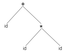
Abstract syntax tree is another name for the syntax tree.

A sentence id + id * id would have the following syntax tree:

Parse Tree 

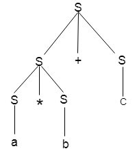
A parse tree is an ordered, rooted tree that represents the syntactic structure of a string according to some context-free grammar. 

Parsing tree, derivation tree, and concrete syntax tree are some other names for parse tree 

Example:

Production

S= S+ S | S * S  

S = a|b|c  

Input:

a * b + c

 

 

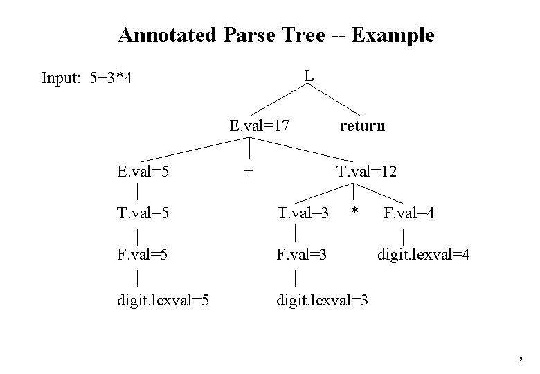
Annotated Parse Tree – The parse tree containing the values of attributes at each node for given input string is called annotated or decorated parse tree.

Features –

• High level specification
• Hides implementation details
• Explicit order of evaluation is not specified

 

Difference

The main difference between parse tree and syntax tree is that parse tree is a hierarchical structure that represents the derivation of the grammar to obtain input strings while syntax tree is a way of representing the syntax of a programming language as a hierarchical tree similar structure.

 Moreover, parse tree contains records of the rules (tokens) to match input texts while syntax tree contains records of the syntax of programming language. Hence, this is another major difference between parse tree and syntax tree.

 

 

Introduction | Structure of a Compiler

Compiler, Computer software that translates (compiles) source code written in a high-level language (e.g., C++) into a set of machine-language instructions that can be understood by a digital computer’s CPU. 

Compilers are very large programs, with error-checking and other abilities. 

Some compilers translate high-level language into an intermediate assembly language, which is then translated (assembled) into machine code by an assembly program or assembler. Other compilers generate machine language directly.

  The Structure of a Compiler

There are two parts: analysis and synthesis.

Analysis (Front End)

• The analysis part breaks up the source program into constituent pieces and imposes a grammatical structure on them.
• It then uses this structure to create an intermediate representation of the source program. 
• If the analysis part detects that the source program is either syntactically ill formed or semantically unsound, then it must provide informative messages, so the user can take corrective action. 
• The analysis part also collects information about the source program and stores it in a data structure called a symbol table , which is passed along with the intermediate representation to the synthesis part.

Synthesis (Back End)

• The synthesis part constructs the desired target program from the intermediate representation and the information in the symbol table.

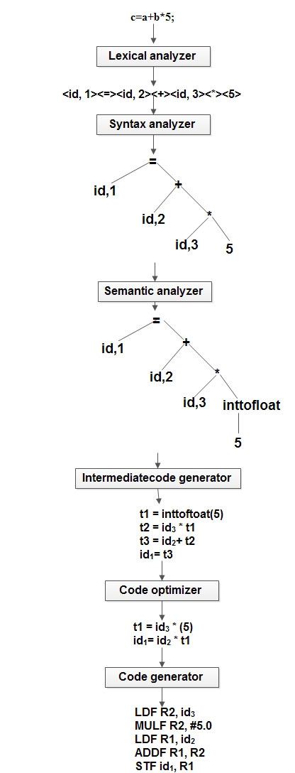
Different Phases

 

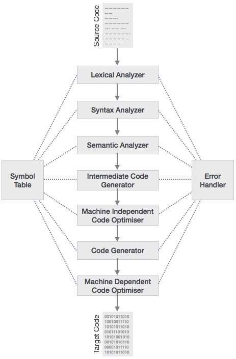
Some compilers have a machine-independent optimization phase between the front end and the back end. The purpose of this optimization phase is to perform transformations on the intermediate representation, so that the back end can produce a better target program than it would have otherwise produced from an unoptimized intermediate representation. Since optimization is optional, one or the other of the two optimization phases will be missing.

1. Lexical Analysis (Scanning)

• The first phase of a compiler is called lexical analysis or scanning . 
• The lexical analyzer reads the stream of characters making up the source program and groups the characters into meaningful sequences called lexemes . 
• For each lexeme, the lexical analyzer produces as output a token(sequence of characters that represent lexical unit) of the form,

 token-name ; attribute-value

that it passes on to the subsequent phase, syntax analysis. 

In the token, the first component token-name is an abstract symbol that is used during syntax analysis, and the second component attribute-value points to an entry in the symbol table for this token. 

Input: stream of characters

Output: Token

example:

ip: position = initial + rate * 60 (lexemes)

op: <id, 1> <=> <id, 2> <+> <id, 3> <*> <60>  (tokens)

2. Syntax Analysis (Parsing)

• The second phase of the compiler is syntax analysis or parsing . 
• The parser uses the first components of the tokens produced by the lexical analyzer to create a tree-like intermediate representation that depicts the grammatical structure of the token stream. 
• A typical representation is a syntax tree in which each interior node represents an operation and the children of the node represent the arguments of the operation.

Input: Tokens

Output: Abstract Syntax tree

 

3. Semantic Analysis

• The semantic analyzer uses the  syntax tree and the information in the symbol table to check the source program for semantic consistency with the language definition. 
• It also gathers type information and saves it in either the syntax tree or the symbol table, for subsequent use during intermediate-code generation.
• Type Checking is taken care of in this phase. This ensures that the variables are assigned values according to their declaration.
  So if a variable have been declared as integer and then assigned a float, the error is trapped by the Semantic Analyzer.
• This phase also identifies chunks of code such as operands and operators of statements in the input code.
  The output of this phase includes the Parse Tree/ Annotated Parse Tree
  
• The language specification may permit some type conversions called coercion .
  

4. Intermediate Code Generation 

Intermediate code generation produces intermediate representations for the source program. This intermediate representation should have two important properties:

It should be easy to produce

It should be easy to translate into the target machine

Different forms of ICG:

     o Post-fix notation

     o Three address code

     o Syntax tree

Most commonly used form is the three address code (It makes use of at most three addresses and one operator to represent an expression and the value computed at each instruction is stored in temporary variable generated by compiler.).

t1 = inttofloat(60)
t2 = id3 * t1
t3 = id2 + t2
id1 = t3

5. Code Optimization  

Code-optimization phase attempts to improve the intermediate code so that better target code will result. Usually better means faster, but other objectives may be desired, such as shorter code, or target code that consumes less power.

In Code Optimization, the code is optimized to remove redundant codes and the optimize for efficient memory management as well as improve the speed of execution. The intermediate code ensures that a target code can be generated for any machine enabling portability across different platforms.
Output of this phase is the Optimized Code.

6. Code Generation

• The code generator takes an intermediate representation of the source program as input and maps it into the target language. 
•  Registers or memory locations are selected for each of the variables used by the program. 
• Then, the intermediate instructions are translated into sequences of machine instructions that perform the same task. 
• A crucial aspect of code generation is the judicious assignment of registers to hold variables.

         LDF R₂, id₃

         MULF R₂, # 60.0

         LDF R₁, id₂

         ADDF R₁, R₂

         STF id₁, R₁

 

Symbol Table Management

• The symbol table is a data structure containing a record for each variable name, with fields for the attributes of the name.
• The data structure should be designed to allow the compiler to find the record for each name quickly and to store or retrieve data from that record quickly 

 

Example