SA algorithm is one of the most preferred heuristic methods for solving optimization problems.
It is a probabilistic technique which is an effective and general form of optimization.
It is useful in finding global optima of a given function when there is lot of local optima.
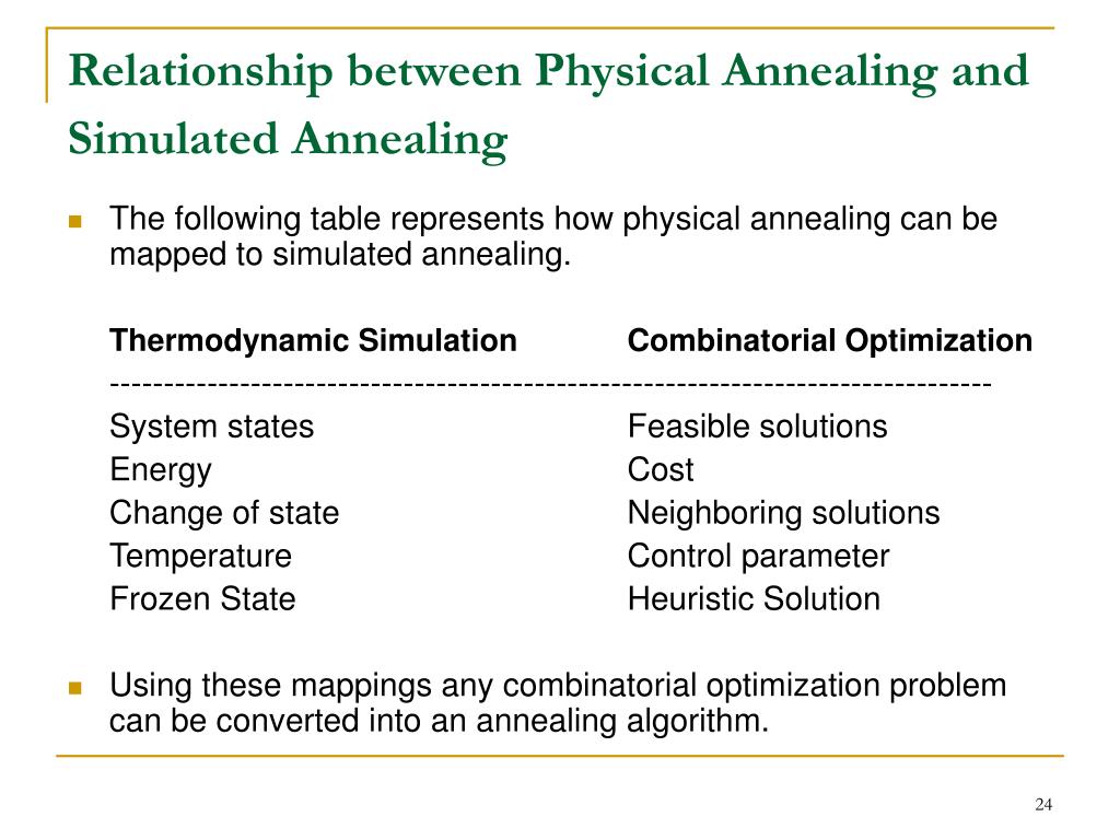
“Annealing” (heat (metal or glass) and allow it to cool slowly, in order to remove internal stresses and toughen it) refers to an analogy with thermodynamics, specifically with the way that metals cool and anneal.
Simulated annealing uses the objective function of an optimization problem instead of the energy of a material.
Simulated annealing is based on metallurgical practices by which a material is heated to a high temperature and cooled. At high temperatures, atoms may shift unpredictably, often eliminating impurities as the material cools into a pure crystal. This is replicated via the simulated annealing optimization algorithm, with energy state corresponding to current solution.
Physical Annealing:
- Simulated Annealing (SA) mimics the Physical Annealing process but is used for optimizing parameters in a model.
- The Simulated Annealing algorithm is based upon Physical Annealing in real life.
- Physical Annealing is the process of heating up a material until it reaches an annealing temperature and then it will be cooled down slowly in order to change the material to a desired structure.
- When the material is hot, the molecular structure is weaker and is more susceptible to change.
- When the material cools down, the molecular structure is harder and is less susceptible to change.
Another important part of this analogy is the following equation from Thermal Dynamics:
This equation calculates the probability that the Energy Magnitude will increase. We can calculate this value given some Energy Magnitude and some temperature t along with the Boltzmann constant k.
Implementation of SA is surprisingly simple. The algorithm is basically hill-climbing except instead of picking the best move, it picks a random move. If the selected move improves the solution, then it is always accepted. Otherwise, the algorithm makes the move anyway with some probability less than 1. The probability decreases exponentially with the “badness” of the move, which is the amount ΔE by which the solution is worsened (i.e., energy is increased.)
Acceptance Criteria
The law of thermodynamics state that at temperature, T, the probability of
an increase in energy of magnitude, ΔE, is given by
P(ΔE) = e−ΔE/kT
where k is a constant that relates temperature to energy known as Boltzmann’s constant.
At higher values of T, uphill moves are more likely to occur. As T tends to zero, they become more and more unlikely, until the algorithm behaves more or less like hill-climbing.
In a typical SA optimization, T starts high and is gradually decreased according to an “annealing schedule”.
A certain number of iterations are carried out at each temperature and then the temperature is decreased. This is repeated until the system freezes into a steady state.
This equation is directly used in simulated annealing, although it is usual to drop the Boltzmann constant as this was only introduced into the equation to cope with different materials. Therefore, the probability of accepting a worse state is given by the equation
P = e−ΔE/T > r
where, ΔE= the change in the evaluation function
T= the current temperature
r= a random number between 0 and 1
The probability of accepting a worse move is a function of both the temperature of the system and of the change in the cost function.
As the temperature of the system decreases the probability of accepting a worse move is decreased. This is the same as gradually moving to a frozen state in physical annealing.
Also if the temperature is zero then only better moves will be accepted which effectively makes simulated annealing act like hill climbing.
Simulated annealing is typically used in discrete, but very large, configuration spaces, such as the set of possible orders of cities in the Traveling Salesman problem and in VLSI routing. It has a broad range of application that is still being explored.
The mapping of time to temperature and how fast the temperature decreases is called the Annealing Schedule.
The algorithm starts initially with set to a high value (or infinity), and then it is decreased at each step following some annealing schedule—which may be specified by the user, but must end with towards the end of the allotted time budget. In this way, the system is expected to wander initially towards a broad region of the search space containing good solutions, ignoring small features of the energy function; then drift towards low-energy regions that become narrower and narrower; and finally move downhill according to the steepest descent heuristic.
For any given finite problem, the probability that the simulated annealing algorithm terminates with a global optimal solution approaches 1 as the annealing schedule is extended. This theoretical result, however, is not particularly helpful, since the time required to ensure a significant probability of success will usually exceed the time required for a complete search of the solution space.
Pseudocode
The following pseudocode presents the simulated annealing heuristic as described above. It starts from a state s0 and continues until a maximum of kmax steps have been taken. In the process, the call neighbour(s) should generate a randomly chosen neighbour of a given state s; the call random(0, 1) should pick and return a value in the range [0, 1], uniformly at random. The annealing schedule is defined by the call temperature(r), which should yield the temperature to use, given the fraction r of the time budget that has been expended so far.
- Let s = s0
- For k = 0 through kmax (exclusive):
- T ← temperature( (k+1)/kmax )
- Pick a random neighbour, snew ← neighbour(s)
- If P(E(s), E(snew), T) ≥ random(0, 1):
- s ← snew
- Output: the final state s
First, generate a random solution
We can do this however we want. The main point is that it's random - it doesn't need to be your best guess at the optimal solution.
Calculate its cost using some cost function you've defined
This, too, is entirely up to you. Depending on your problem, it might be as simple as counting the total number of miles the traveling salesman's traveled. Or it might be an incredibly complex melding of multiple factors. Calculating the cost of each solution is often the most expensive part of the
algorithm, so it pays to keep it simple.
Generate a random neighboring solution
"Neighboring" means there's only one thing that differs between the old solution and the new solution. Effectively, you switch two elements of your solution and recalculate the cost. The main requirement is that it be done randomly.
Calculate the new solution's cost
Use the same cost function as above. You can see why it needs to perform well - it gets called with each iteration of the algorithm.
If cnew < cold: move to the new solution
If the new solution has a smaller cost than the old solution, the new one is better. This makes the algorithm happy - it's getting closer to an optimum. It will "move" to that new solution, saving it as the base for its next iteration.
If cnew > cold: maybe move to the new solution
This is where things get interesting. Most of the time, the algorithm will avoid moving to a worse solution. If it did that all of the time, though, it would get caught at local maxima. To avoid that problem, it sometimes elects to keep the worse solution. To decide, the algorithm calculates something called the 'acceptance probability' and then compares it to a random number.
#Selecting the parameters
In order to apply the simulated annealing method to a specific problem, one must specify the following parameters:- state space,
- energy
(goal) function
E(), - candidate generator procedure
neighbour(), - acceptance probability function
P(), - annealing schedule
temperature() - initial temperature <init temp>.
Parameter setting is the significant part to the algorithm
s and e to sbest and ebest
and perhaps restart the annealing schedule. The decision to restart
could be based on several criteria. Notable among these include
restarting based on a fixed number of steps, based on whether the
current energy is too high compared to the best energy obtained so far,
restarting randomly, etc.


Some Example of Problems to Optimize with SA
- Travelling Salesman Problem (TSP)
- Scheduling Problems
- Task Allocations
- Graph colouring and partitioning
- Non-linear function optimizations
Applications
Circuit Partitioning & Placement
Hardware/Software Partitioning
Graph Partitioning
VLSI: Placement, routing
Image Processing
Strategy Scheduling for capital products with complex product structure
Umpire scheduling in US open tournament
Event-based learning situations
Advantages vs. Disadvantages of SA
Advantages
- Easy to implement and use
- Provides optimal solutions to a wide range of problems
Disadvantages
- Can take a long time to run if the annealing schedule is very long
- There are a lot of tuneable parameters in this algorithm
Practical Issues
The maximum temperature
Scheme for decreasing temperature
Strategy for proposing updates
Simulated Annealing versus Hill Climbing
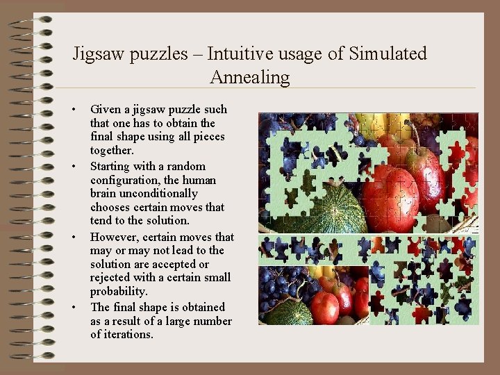
- Hill climbing suffers from problems in getting stuck at local minima (or maxima). Simulated annealing solves this problem by allowing worse moves (lesser quality) to be taken some of the time. That is, it allows some uphill steps so that it can escape from local minima.
- Unlike hill climbing, simulated annealing chooses a random move from the neighbourhood (recall that hill climbing chooses the best move from all those available).
- If the move is better than its current position then simulated annealing will always take it.
- If the move is worse (i.e. lesser quality) then it will be accepted based on some probability.

REF
https://www.geeksforgeeks.org/simulated-annealing/
https://en.wikipedia.org/wiki/Simulated_annealing
https://www.sciencedirect.com/topics/engineering/simulated-annealing-algorithm
https://towardsdatascience.com/optimization-techniques-simulated-annealing-d6a4785a1de7


