Hadoop Input/output formats & Setting up a Hadoop cluster

Hadoop InputFormat

• InputFormatdefines, How the input files are split up and read in Hadoop. 
• An Hadoop InputFormat is the first component in Map-Reduce, it is responsible for creating the input splits and dividing them into records. 
• Initially, the data for a MapReduce task is stored in input files, and input files typically reside in HDFS.
• Although these files format is arbitrary, line-based log files and binary format can be used. 
• Using InputFormat we define how these input files are split and read. 
• The InputFormat class is one of the fundamental classes in the Hadoop MapReduce framewor.

Types of InputFormat in MapReduce

1. FileInputFormat in Hadoop

It is the base class for all file-based InputFormats. Hadoop FileInputFormat specifies input directory where data files are located. When we start a Hadoop job, FileInputFormat is provided with a path containing files to read. FileInputFormat will read all files and divides these files into one or more InputSplits.

2. TextInputFormat

It is the default InputFormat of MapReduce. TextInputFormat treats each line of each input file as a separate record and performs no parsing. This is useful for unformatted data or line-based records like log files.

• Key – It is the byte offset of the beginning of the line within the file (not whole file just one split), so it will be unique if combined with the file name.
• Value – It is the contents of the line, excluding line terminators.

3. KeyValueTextInputFormat

It is similar to TextInputFormat as it also treats each line of input as a separate record. While TextInputFormat treats entire line as the value, but the KeyValueTextInputFormat breaks the line itself into key and value by a tab character (‘/t’). Here Key is everything up to the tab character while the value is the remaining part of the line after tab character.

4. SequenceFileInputFormat

Hadoop SequenceFileInputFormat is an InputFormat which reads sequence files. Sequence files are binary files that stores sequences of binary key-value pairs. Sequence files block-compress and provide direct serialization and deserialization of several arbitrary data types (not just text). Here Key & Value both are user-defined.

5. SequenceFileAsTextInputFormat

Hadoop SequenceFileAsTextInputFormat is another form of SequenceFileInputFormat which converts the sequence file key values to Text objects. By calling ‘tostring()’ conversion is performed on the keys and values. This InputFormat makes sequence files suitable input for streaming.

6. SequenceFileAsBinaryInputFormat

Hadoop SequenceFileAsBinaryInputFormat is a SequenceFileInputFormat using which we can extract the sequence file’s keys and values as an opaque binary object.

7. NLineInputFormat

Hadoop NLineInputFormat is another form of TextInputFormat where the keys are byte offset of the line and values are contents of the line. Each mapper receives a variable number of lines of input with TextInputFormat and KeyValueTextInputFormat and the number depends on the size of the split and the length of the lines. And if we want our mapper to receive a fixed number of lines of input, then we use NLineInputFormat.
N is the number of lines of input that each mapper receives. By default (N=1), each mapper receives exactly one line of input. If N=2, then each split contains two lines. One mapper will receive the first two Key-Value pairs and another mapper will receive the second two key-value pairs.

8. DBInputFormat

Hadoop DBInputFormat is an InputFormat that reads data from a relational database, using JDBC. As it doesn’t have portioning capabilities, so we need to careful not to swamp the database from which we are reading too many mappers. So it is best for loading relatively small datasets, perhaps for joining with large datasets from HDFS using MultipleInputs. Here Key is LongWritables while Value is DBWritables.

Hadoop Output Format

As we know, Reducer takes as input a set of an intermediate key-value pair produced by the mapper and runs a reducer function on them to generate output that is again zero or more key-value pairs.

RecordWriter writes these output key-value pairs from the Reducer phase to output files.

Types of Hadoop Output Formats

i. TextOutputFormat

MapReduce default Hadoop reducer Output Format is TextOutputFormat, which writes (key, value) pairs on individual lines of text files and its keys and values can be of any type since TextOutputFormat turns them to string by calling toString() on them. Each key-value pair is separated by a tab character, which can be changed using MapReduce.output.textoutputformat.separator property. KeyValueTextOutputFormat is used for reading these output text files since it breaks lines into key-value pairs based on a configurable separator.

ii. SequenceFileOutputFormat

It is an Output Format which writes sequences files for its output and it is intermediate format use between MapReduce jobs, which rapidly serialize arbitrary data types to the file; and the corresponding SequenceFileInputFormat will deserialize the file into the same types and presents the data to the next mapper in the same manner as it was emitted by the previous reducer, since these are compact and readily compressible. Compression is controlled by the static methods on SequenceFileOutputFormat.

iii. SequenceFileAsBinaryOutputFormat

It is another form of SequenceFileInputFormat which writes keys and values to sequence file in binary format.

iv. MapFileOutputFormat

It is another form of FileOutputFormat in Hadoop Output Format, which is used to write output as map files. The key in a MapFile must be added in order, so we need to ensure that reducer emits keys in sorted order.
Any doubt yet in Hadoop Oputput Format? Please Ask.

v. MultipleOutputs

It allows writing data to files whose names are derived from the output keys and values, or in fact from an arbitrary string.

vi. LazyOutputFormat

Sometimes FileOutputFormat will create output files, even if they are empty. LazyOutputFormat is a wrapper OutputFormat which ensures that the output file will be created only when the record is emitted for a given partition.

vii. DBOutputFormat

DBOutputFormat in Hadoop is an Output Format for writing to relational databases and HBase. It sends the reduce output to a SQL table. It accepts key-value pairs, where the key has a type extending DBwritable. Returned RecordWriter writes only the key to the database with a batch SQL query.

 REF

https://data-flair.training/blogs/hadoop-inputformat/

https://data-flair.training/blogs/hadoop-outputformat/

 https://www.edureka.co/blog/hadoop-clusters

MapReduce framework

 Hadoop HDFS stores the data, MapReduce processes the data stored in HDFS, and YARN divides the tasks and assigns resources.

•  MapReduce is a software framework and programming model that allows us to perform distributed and parallel processing on large data sets in a distributed environment

• It is the processing unit in Hadoop.
• MapReduce consists of two distinct tasks – Map and Reduce 
•  It works by dividing the task into independent subtasks and executes them in parallel across various DataNodes thereby increasing the throughput,fially
• Map tasks deal with splitting and mapping of data while Reduce tasks shuffle and reduce the data. 
• Hadoop is capable of running MapReduce programs written in various languages: Java, Ruby, Python, and C++. 
• The input to each phase is key-value pairs.  The type of key, value pairs is specified by the programmer through the InputFormat class. By default, the text input format is used. 
  

• The first is the map job, where a block of data is read and processed to produce key-value pairs as intermediate outputs.
• The output of a Mapper or map job (key-value pairs) is input to the Reducer.
• The reducer receives the key-value pair from multiple map jobs.
• Then, the reducer aggregates those intermediate data tuples (intermediate key-value pair) into a smaller set of tuples or key-value pairs which is the final output.
  

MapReduce Architecture

Basic strategy: divide & conquer
Partition a large problem into smaller subproblems, to the extent that subproblems are independent.

The whole process goes through four phases of execution namely, splitting, mapping, shuffling, and reducing.

 

 

The data goes through the following phases of MapReduce in Big Data

Spliting

An input to a MapReduce in Big Data job is divided into fixed-size pieces called input splits Input split is a chunk of the input that is consumed by a single map

Mapping

• This is the very first phase in the execution of map-reduce program. 
• In this phase data in each split is passed to a mapping function to produce output values.

Shuffling

• This phase consumes the output of Mapping phase. 
• Its task is to consolidate the relevant records from Mapping phase output. 
• In our example, the same words are clubbed together along with their respective frequency.

Reducing

• In this phase, output values from the Shuffling phase are aggregated.
• This phase combines values from Shuffling phase and returns a single output value. 
• In short, this phase summarizes the complete dataset.

 

How MapReduce Organizes Work?

Hadoop divides the job into tasks. There are two types of tasks:

1. Map tasks (Splits & Mapping)
2. Reduce tasks (Shuffling, Reducing)

The complete execution process (execution of Map and Reduce tasks, both) is controlled by two types of entities called a

1. Jobtracker: Acts like a master (responsible for complete execution of submitted job)
2. Multiple Task Trackers: Acts like slaves, each of them performing the job

For every job submitted for execution in the system, there is one Jobtracker that resides on Namenode and there are multiple tasktrackers which reside on Datanode.

 

Working of Hadoop MapReduce

• A job is divided into multiple tasks which are then run onto multiple data nodes in a cluster.
• It is the responsibility of job tracker to coordinate the activity by scheduling tasks to run on different data nodes.
• Execution of individual task is then to look after by task tracker, which resides on every data node executing part of the job.
• Task tracker's responsibility is to send the progress report to the job tracker.
• In addition, task tracker periodically sends 'heartbeat' signal to the Jobtracker so as to notify him of the current state of the system. 
• Thus job tracker keeps track of the overall progress of each job. In the event of task failure, the job tracker can reschedule it on a different task tracker.

Advantages of MapReduce

The two biggest advantages of MapReduce are:

      1. Parallel Processing:

In MapReduce, we are dividing the job among multiple nodes and each node works with a part of the job simultaneously. So, MapReduce is based on Divide and Conquer paradigm which helps us to process the data using different machines. As the data is processed by multiple machines instead of a single machine in parallel, the time taken to process the data gets reduced by a tremendous amount

2. Data Locality: 

Instead of moving data to the processing unit, we are moving the processing unit to the data in the MapReduce Framework.  In the traditional system, we used to bring data to the processing unit and process it. But, as the data grew and became very huge, bringing this huge amount of data to the processing unit posed the following issues: 

• Moving huge data to processing is costly and deteriorates the network performance. 
• Processing takes time as the data is processed by a single unit which becomes the bottleneck.
• The master node can get over-burdened and may fail.  

Now, MapReduce allows us to overcome the above issues by bringing the processing unit to the data. So, as you can see in the above image that the data is distributed among multiple nodes where each node processes the part of the data residing on it. This allows us to have the following advantages:

• It is very cost-effective to move processing unit to the data.
• The processing time is reduced as all the nodes are working with their part of the data in parallel.
• Every node gets a part of the data to process and therefore, there is no chance of a node getting overburdened.
  

Why MapReduce?

Traditional Enterprise Systems normally have a centralized server to store and process data. The following illustration depicts a schematic view of a traditional enterprise system. Traditional model is certainly not suitable to process huge volumes of scalable data and cannot be accommodated by standard database servers. Moreover, the centralized system creates too much of a bottleneck while processing multiple files simultaneously.

Google solved this bottleneck issue using an algorithm called MapReduce. MapReduce divides a task into small parts and assigns them to many computers. Later, the results are collected at one place and integrated to form the result dataset.

MapReduce-Example

Let us take a real-world example to comprehend the power of MapReduce. Twitter receives around 500 million tweets per day, which is nearly 3000 tweets per second. The following illustration shows how Tweeter manages its tweets with the help of MapReduce.

As shown in the illustration, the MapReduce algorithm performs the following actions −

• Tokenize − Tokenizes the tweets into maps of tokens and writes them as key-value pairs.

• Filter − Filters unwanted words from the maps of tokens and writes the filtered maps as key-value pairs.

• Count − Generates a token counter per word.

• Aggregate Counters − Prepares an aggregate of similar counter values into small manageable units.

MapReduce - Algorithm

The MapReduce algorithm contains two important tasks, namely Map and Reduce.

• The map task is done by means of Mapper Class
• The reduce task is done by means of Reducer Class.

Mapper class takes the input, tokenizes it, maps and sorts it. The output of Mapper class is used as input by Reducer class, which in turn searches matching pairs and reduces them.

MapReduce implements various mathematical algorithms to divide a task into small parts and assign them to multiple systems. In technical terms, MapReduce algorithm helps in sending the Map & Reduce tasks to appropriate servers in a cluster.

These mathematical algorithms may include the following −

• Sorting
• Searching
• Indexing
• TF-IDF

Sorting

Sorting is one of the basic MapReduce algorithms to process and analyze data. MapReduce implements sorting algorithm to automatically sort the output key-value pairs from the mapper by their keys.

• Sorting methods are implemented in the mapper class itself.

• In the Shuffle and Sort phase, after tokenizing the values in the mapper class, the Context class (user-defined class) collects the matching valued keys as a collection.

• To collect similar key-value pairs (intermediate keys), the Mapper class takes the help of RawComparator class to sort the key-value pairs.

• The set of intermediate key-value pairs for a given Reducer is automatically sorted by Hadoop to form key-values (K2, {V2, V2, …}) before they are presented to the Reducer.

Searching

Searching plays an important role in MapReduce algorithm. It helps in the combiner phase (optional) and in the Reducer phase. Let us try to understand how Searching works with the help of an example.

Example

The following example shows how MapReduce employs Searching algorithm to find out the details of the employee who draws the highest salary in a given employee dataset.

• Let us assume we have employee data in four different files − A, B, C, and D. Let us also assume there are duplicate employee records in all four files because of importing the employee data from all database tables repeatedly. See the following illustration.

• The Map phase processes each input file and provides the employee data in key-value pairs (<k, v> : <emp name, salary>). See the following illustration.

• The combiner phase (searching technique) will accept the input from the Map phase as a key-value pair with employee name and salary. Using searching technique, the combiner will check all the employee salary to find the highest salaried employee in each file. See the following snippet.

<k: employee name, v: salary>
Max= the salary of an first employee. Treated as max salary

if(v(second employee).salary > Max){
   Max = v(salary);
}

else{
   Continue checking;
}

The expected result is as follows −

<satish, 26000> <gopal, 50000> <kiran, 45000> <manisha, 45000>

• Reducer phase − Form each file, you will find the highest salaried employee. To avoid redundancy, check all the <k, v> pairs and eliminate duplicate entries, if any. The same algorithm is used in between the four <k, v> pairs, which are coming from four input files. The final output should be as follows −

<gopal, 50000>

Indexing

Normally indexing is used to point to a particular data and its address. It performs batch indexing on the input files for a particular Mapper.

The indexing technique that is normally used in MapReduce is known as inverted index. Search engines like Google and Bing use inverted indexing technique. Let us try to understand how Indexing works with the help of a simple example.

Example

The following text is the input for inverted indexing. Here T[0], T[1], and t[2] are the file names and their content are in double quotes.

T[0] = "it is what it is"
T[1] = "what is it"
T[2] = "it is a banana"

After applying the Indexing algorithm, we get the following output −

"a": {2}
"banana": {2}
"is": {0, 1, 2}
"it": {0, 1, 2}
"what": {0, 1}

Here "a": {2} implies the term "a" appears in the T[2] file. Similarly, "is": {0, 1, 2} implies the term "is" appears in the files T[0], T[1], and T[2].

TF-IDF

TF-IDF is a text processing algorithm which is short for Term Frequency − Inverse Document Frequency. It is one of the common web analysis algorithms. Here, the term 'frequency' refers to the number of times a term appears in a document.

Term Frequency (TF)

It measures how frequently a particular term occurs in a document. It is calculated by the number of times a word appears in a document divided by the total number of words in that document.

TF(the) = (Number of times term the ‘the’ appears in a document) / (Total number of terms in the document)

Inverse Document Frequency (IDF)

It measures the importance of a term. It is calculated by the number of documents in the text database divided by the number of documents where a specific term appears.

While computing TF, all the terms are considered equally important. That means, TF counts the term frequency for normal words like “is”, “a”, “what”, etc. Thus we need to know the frequent terms while scaling up the rare ones, by computing the following −

IDF(the) = log_e(Total number of documents / Number of documents with term ‘the’ in it).

The algorithm is explained below with the help of a small example.

Example

Consider a document containing 1000 words, wherein the word hive appears 50 times. The TF for hive is then (50 / 1000) = 0.05.

Now, assume we have 10 million documents and the word hive appears in 1000 of these. Then, the IDF is calculated as log(10,000,000 / 1,000) = 4.

The TF-IDF weight is the product of these quantities − 0.05 × 4 = 0.20.

 REF

https://www.guru99.com/introduction-to-mapreduce.html 

Data Analytics Lifecycle

The Data Analytics Lifecycle is a cyclic process which explains, in six stages, how information in made, collected, processed, implemented, and analyzed for different objectives.

 

 

1. Data Discovery

• This is the initial phase to set your project's objective
• Start with defining your business domain and ensure you have enough resources (time, technology, data, and people) to achieve your goals.
• The biggest challenge in this phase is to accumulate enough information. You need to draft an analytic plan, which requires some serious leg work.

Accumulate resources

First, you have to analyze the models you have intended to develop. Then determine how much domain knowledge you need to acquire for fulfilling those models.

The next important thing to do is assess whether you have enough skills and resources to bring your projects to fruition.

Frame the issue

Problems are most likely to occur while meeting your client's expectations. Therefore, you need to identify the issues related to the project and explain them to your clients. This process is called "framing." You have to prepare a problem statement explaining the current situation and challenges that can occur in the future. You also need to define the project's objective, including the success and failure criteria for the project.

Formulate initial hypothesis

Once you gather all the clients' requirements, you have to develop initial hypotheses after exploring the initial data.

2. Data Preparation and Processing

The Data preparation and processing phase involves collecting, processing, and conditioning data before moving to the model building process.

Identify data sources

You have to identify various data sources and analyze how much and what kind of data you can accumulate within a given time frame. Evaluate the data structures, explore their attributes and acquire all the tools needed.

Collection of data

You can collect data using three methods:

#Data acquisition: You can collect data through external sources.

#Data Entry: You can prepare data points through digital systems or manual entry as well.

#Signal reception: You can accumulate data from digital devices such as IoT devices and control systems.

3. Model Planning

This is a phase where you have to analyze the quality of data and find a suitable model for your project.

This phase needs the availability of an analytic sandbox for the team to work with data and perform analytics throughout the project duration. The team can load data in several ways.

o  Extract, Transform, Load (ETL) – It transforms the data based on a set of business rules before loading it into the sandbox.

o  Extract, Load, Transform (ELT) – It loads the data into the sandbox and then transforms it based on a set of business rules.

o  Extract, Transform, Load, Transform (ETLT) – It’s the combination of ETL and ELT and has two transformation levels.

An analytics sandbox is a part of data lake architecture that allows you to store and process large amounts of data. It can efficiently process a large range of data such as big data, transactional data, social media data, web data, and many more. It is an environment that allows your analysts to schedule and process data assets using the data tools of their choice. The best part of the analytics sandbox is its agility. It empowers analysts to process data in real-time and get essential information within a short duration.

4. Model Building

• Model building is the process where you have to deploy the planned model in a real-time environment. 
• It allows analysts to solidify their decision-making process by gain in-depth analytical information. This is a repetitive process, as you have to add new features as required by your customers constantly.

In this phase, the team develops testing, training, and production datasets. Further, the team builds and executes models meticulously as planned during the model planning phase. They test data and try to find out answers to the given objectives. They use various statistical modeling methods such as regression techniques, decision trees, random forest modeling, and neural networks and perform a trial run to determine whether it corresponds to the datasets.

5. Result Communication and Publication

This is the phase where you have to communicate the data analysis with your clients. It requires several intricate processes where you how to present information to clients in a lucid manner. Your clients don't have enough time to determine which data is essential. Therefore, you must do an impeccable job to grab the attention of your clients.

Check the data accuracy

Is the data provide information as expected? If not, then you have to run some other processes to resolve this issue. You need to ensure the data you process provides consistent information. This will help you build a convincing argument while summarizing your findings.

Highlight important findings

Well, each data holds a significant role in building an efficient project. However, some data inherits more potent information that can truly serve your audience's benefits. While summarizing your findings, try to categorize data into different key points.

Determine the most appropriate communication format

How you communicate your findings tells a lot about you as a professional. We recommend you to go for visuals presentation and animations as it helps you to convey information much faster. However, sometimes you also need to go old-school as well. For instance, your clients may have to carry the findings in physical format. They may also have to pick up certain information and share them with others.

6. Operationalize

As soon you prepare a detailed report including your key findings, documents, and briefings, your data analytics life cycle almost comes close to the end. The next step remains the measure the effectiveness of your analysis before submitting the final reports to your stakeholders.

In this process, you have to move the sandbox data and run it in a live environment. Then you have to closely monitor the results, ensuring they match with your expected goals. If the findings fit perfectly with your objective, then you can finalize the report. Otherwise, you have to take a step back in your data analytics lifecycle and make some changes.

 

Big Data Mining

Big Data Mining: Data Mining with Big Data, Issues, Case Study, Clustering on Big Data, Limitations of Mapreduce Framework, Case Study-Graph Algorithms on Mapreduce

Hierarchical Clustering

 Hierarchical Methods 
This method creates a hierarchical decomposition of the given set of data objects. In data mining and statistics, hierarchical clustering (also called hierarchical cluster analysis or HCA) is a method of cluster analysis which seeks to build a hierarchy of clusters. Strategies for hierarchical clustering generally fall into two types:

• Agglomerative: This is a "bottom-up" approach: each observation starts in its own cluster, and pairs of clusters are merged as one moves up the hierarchy.  
• Divisive: This is a "top-down" approach: all observations start in one cluster, and splits are performed recursively as one moves down the hierarchy.

In general, the merges and splits are determined in a greedy manner. The results of hierarchical clustering are usually presented in a dendrogram (A Dendrogram is a type of tree diagram showing hierarchical relationships between different sets of data).

Agglomerative Hierarchical Clustering

The Agglomerative Hierarchical Clustering is the most common type of hierarchical clustering used to group objects in clusters based on their similarity. It’s also known as AGNES (Agglomerative Nesting). It's a “bottom-up” approach: each observation starts in its own cluster, and pairs of clusters are merged as one moves up the hierarchy.

How does it work?

1. Make each data point a single-point cluster → forms N clusters
2. Take the two closest data points and make them one cluster → forms N-1 clusters
3. Take the two closest clusters and make them one cluster → Forms N-2 clusters.
4. Repeat step-3 until you are left with only one cluster.

Pseudo Code Steps:

1. Begin with n clusters, each containing one object and we will number the clusters 1 through n.
2. Compute the between-cluster distance D(r, s) as the between-object distance of the two objects in r and s respectively, r, s =1, 2, ..., n. Let the square matrix D = (D(r, s)). If the objects are represented by quantitative vectors we can use Euclidean distance.
3. Next, find the most similar pair of clusters r and s, such that the distance, D(r, s), is minimum among all the pairwise distances.
4. Merge r and s to a new cluster t and compute the between-cluster distance D(t, k) for any existing cluster k ≠ r, s . Once the distances are obtained,  delete the rows and columns corresponding to the old cluster r and s in the D matrix, because r and s do not exist anymore. Then add a new row and column in D corresponding to cluster t.
5. Repeat Step 3 a total of n − 1 times until there is only one cluster left.

 

There are several ways to measure the distance between clusters in order to decide the rules for clustering, and they are often called Linkage Methods. Some of the common linkage methods are:

• Complete-linkage: the distance between two clusters is defined as the longest distance between two points in each cluster.
• Single-linkage: the distance between two clusters is defined as the shortest distance between two points in each cluster. This linkage may be used to detect high values in your dataset which may be outliers as they will be merged at the end.
• Average-linkage: the distance between two clusters is defined as the average distance between each point in one cluster to every point in the other cluster.
• Centroid-linkage: finds the centroid of cluster 1 and centroid of cluster 2, and then calculates the distance between the two before merging.
  

Divisive Hierarchical Clustering

In Divisive or DIANA(DIvisive ANAlysis Clustering) is a top-down clustering method where we assign all of the observations to a single cluster and then partition the cluster to two least similar clusters. Finally, we proceed recursively on each cluster until there is one cluster for each observation. So this clustering approach is exactly opposite to Agglomerative clustering.

There is evidence that divisive algorithms produce more accurate hierarchies than agglomerative algorithms in some circumstances but is conceptually more complex.

In both agglomerative and divisive hierarchical clustering, users need to specify the desired number of clusters as a termination condition(when to stop merging).

 

https://en.wikipedia.org/wiki/Hierarchical_clustering

https://www.kdnuggets.com/2019/09/hierarchical-clustering.html 

Data Stores || NoSqL Stores

Data Storage: NoSQL Stores , Key-Value Stores , Columnar Stores ,
Document Stores ,Graph Databases ,Case Studies , HDFS, HBase, Hive,
MongoDB, Neo4j

Role of Data Scientist & Big Data Sources

Role of Data Scientist

“Start-ups are producing so much data that hiring has increased dramatically. Salaries are on the rise for data scientists who are able to work closely with developers to provide value to end users,".

• The role of a data scientist is becoming more pivotal to even traditional organizations who didn’t previously invest much of their budgets in technology positions. 
• Big data is changing the way old-school organizations conduct business and manage marketing, and the data scientist is at the center of that transformation.
• Data scientists are often experts in technologies such as Hadoop, Pig, Python, and Java. Their jobs can focus on data management, analytics modeling, and business analysis. Because they tend to specialize in a narrow niche of data science, data scientists often work in teams within a company.
• Data scientists can be real change-makers within an organization, offering insight that can illuminate the company’s trajectory toward its ultimate business goals. 
• Data scientists are integral to supporting both leaders and developers in creating better products and paradigms. And as their role in big business becomes more and more important, they are in increasingly short supply.

Big Data Sources

The bulk of big data generated comes from three primary sources: social data, machine data and transactional data.

Social data comes from the Likes, Tweets & Retweets, Comments, Video Uploads, and general media that are uploaded and shared via the world’s favorite social media platforms. This kind of data provides invaluable insights into consumer behavior and sentiment and can be enormously influential in marketing analytics. The public web is another good source of social data, and tools like Google Trends can be used to good effect to increase the volume of big data.

Machine data is defined as information which is generated by industrial equipment, sensors that are installed in machinery, and even web logs which track user behavior. This type of data is expected to grow exponentially as the internet of things grows ever more pervasive and expands around the world. Sensors such as medical devices, smart meters, road cameras, satellites, games and the rapidly growing Internet Of Things will deliver high velocity, value, volume and variety of data in the very near future.

Transactional data is generated from all the daily transactions that take place both online and offline. Invoices, payment orders, storage records, delivery receipts – all are characterized as transactional data yet data alone is almost meaningless, and most organizations struggle to make sense of the data that they are generating and how it can be put to good use.

Introduction to BigData

Every day, we create roughly 2.5 quintillion bytes of data

• 500 million tweets are sent
• 294 billion emails are sent
• 4 petabytes of data are created on Facebook
• 4 terabytes of data are created from each connected car
• 65 billion messages are sent on WhatsApp
• 5 billion searches are made

Big Data is a collection of data that is huge in volume, yet growing exponentially with time.

It is a data with so large size and complexity that none of traditional data management tools can store it or process it efficiently. Big data is also a data but with huge size.

Data: The quantities, characters, or symbols on which operations are performed by a computer, which may be stored and transmitted in the form of electrical signals and recorded on magnetic, optical, or mechanical recording media. 

Examples Of Big Data

* The New York Stock Exchange generates about one terabyte of new trade data per day.

* Social Media: The statistic shows that 500+terabytes of new data get ingested into the databases of social media site Facebook, every day. This data is mainly generated in terms of photo and video uploads, message exchanges, putting comments etc.

* A single Jet engine can generate 10+terabytes of data in 30 minutes of flight time. With many thousand flights per day, generation of data reaches up to many Petabytes.

Characteristics Of Big Data

Big data can be described by the following characteristics:

• Volume (Scale of data)
  
• Variety (Forms of data)
• Velocity (Analysis of data flow)
  
• Veracity (Uncertainty of data)
• Value 
• Unfortunately, sometimes volatility isn’t within our control. The volatility, sometimes referred to as another “V” of big data, is the rate of change and lifetime of the data

Volume  

• The name Big Data itself is related to a size which is enormous. 
• Size of data plays a very crucial role in determining value out of data. 
• Also, whether a particular data can actually be considered as a Big Data or not, is dependent upon the volume of data. 
• Hence, 'Volume' is one characteristic which needs to be considered while dealing with Big Data.

As an example of a high-volume dataset, think about Facebook. The world’s most popular social media platform now has more than 2.2 billion active users, many of whom spend hours each day posting updates, commenting on images, liking posts, clicking on ads, playing games, and doing a zillion other things that generate data that can be analyzed. This is high-volume big data in no uncertain terms.

Variety 

• Variety refers to heterogeneous sources and the nature of data, both structured and unstructured. 
• During earlier days, spreadsheets and databases were the only sources of data considered by most of the applications. 
• Nowadays, data in the form of emails, photos, videos, monitoring devices, PDFs, audio, etc. are also being considered in the analysis applications. 
• This variety of unstructured data poses certain issues for storage, mining and analyzing data.

Facebook, of course, is just one source of big data. Imagine just how much data can be sourced from a company’s website traffic, from review sites, social media (not just Facebook, but Twitter, Pinterest, Instagram, and all the rest of the gang as well), email, CRM systems, mobile data, Google Ads – you name it. All these sources (and many more besides) produce data that can be collected, stored, processed and analyzed. When combined, they give us our second characteristic – variety. Variety, indeed, is what makes it really, really big. Data scientists and analysts aren’t just limited to collecting data from just one source, but many. And this data can be broken down into three distinct types – structured, semi-structured, and unstructured.

Velocity 

• The term 'velocity' refers to the speed of generation of data. 
• How fast the data is generated and processed to meet the demands, determines real potential in the data.
• Big Data Velocity deals with the speed at which data flows in from sources like business processes, application logs, networks, and social media sites, sensors, Mobile devices, etc. 
• The flow of data is massive and continuous.

Facebook messages, Twitter posts, credit card swipes and ecommerce sales transactions are all examples of high velocity data.

Veracity 

This refers to the inconsistency which can be shown by the data at times, thus hampering the process of being able to handle and manage the data effectively. 

Veracity refers to the quality, accuracy and trustworthiness of data that’s collected. As such, veracity is not necessarily a distinctive characteristic of big data (as even little data needs to be trustworthy), but due to the high volume, variety and velocity, high reliability is of paramount importance if a business is draw accurate conclusions from it. High veracity data is the truly valuable stuff that contributes in a meaningful way to overall results. And it needs to be high quality. 

Value
Value sits right at the top of the pyramid and refers to an organization’s ability to transform those tsunamis of data into real business. With all the tools available today, pretty much any enterprise can get started with big data

Types Of Big Data

Following are the types of Big Data:

1. Structured
2. Unstructured
3. Semi-structured

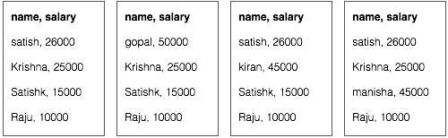
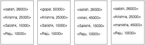
Structured

By structured data, we mean data that can be processed, stored, and retrieved in a fixed format. It refers to highly organized information that can be readily and seamlessly stored and accessed from a database by simple search engine algorithms. For instance, the employee table in a company database will be structured as the employee details, their job positions, their salaries, etc., will be present in an organized manner. 

Unstructured

Unstructured data refers to the data that lacks any specific form or structure whatsoever. This makes it very difficult and time-consuming to process and analyze unstructured data. Email is an example of unstructured data. Structured and unstructured are two important types of big data.

Semi-structured

Semi structured is the third type of big data. Semi-structured data pertains to the data containing both the formats mentioned above, that is, structured and unstructured data. To be precise, it refers to the data that although has not been classified under a particular repository (database), yet contains vital information or tags that segregate individual elements within the data.

 Importance

Ability to process Big Data brings in multiple benefits, such as-

Businesses can utilize outside intelligence while taking decisions- Access to social data from search engines and sites like facebook, twitter are enabling organizations to fine tune their business strategies.

Improved customer service- Traditional customer feedback systems are getting replaced by new systems designed with Big Data technologies. In these new systems, Big Data and natural language processing technologies are being used to read and evaluate consumer responses.

Early identification of risk to the product/services, if any

Better operational efficiency- Big Data technologies can be used for creating a staging area or landing zone for new data before identifying what data should be moved to the data warehouse. In addition, such integration of Big Data technologies and data warehouse helps an organization to offload infrequently accessed data.

Advantages of Big Data (Features)

• • Opportunities to Make Better Decisions. ...
  • Increasing Productivity and Efficiency. ...
  • Reducing Costs. ...
  • Improving Customer Service and Customer Experience. ...
  • Fraud and Anomaly Detection. ...
  • Greater Agility and Speed to Market. ...
  • Questionable Data Quality. ...
  • Heightened Security Risks.
   
• One of the biggest advantages of Big Data is predictive analysis. Big Data analytics tools can predict outcomes accurately, thereby, allowing businesses and organizations to make better decisions, while simultaneously optimizing their operational efficiencies and reducing risks.
• By harnessing data from social media platforms using Big Data analytics tools, businesses around the world are streamlining their digital marketing strategies to enhance the overall consumer experience. Big Data provides insights into the customer pain points and allows companies to improve upon their products and services.
• Being accurate, Big Data combines relevant data from multiple sources to produce highly actionable insights. Almost 43% of companies lack the necessary tools to filter out irrelevant data, which eventually costs them millions of dollars to hash out useful data from the bulk. Big Data tools can help reduce this, saving you both time and money.
• Big Data analytics could help companies generate more sales leads which would naturally mean a boost in revenue. Businesses are using Big Data analytics tools to understand how well their products/services are doing in the market and how the customers are responding to them. Thus, the can understand better where to invest their time and money.
• With Big Data insights, you can always stay a step ahead of your competitors. You can screen the market to know what kind of promotions and offers your rivals are providing, and then you can come up with better offers for your customers. Also, Big Data insights allow you to learn customer behavior to understand the customer trends and provide a highly ‘personalized’ experience to them.   

Applications

1) Healthcare 

• Big Data has already started to create a huge difference in the healthcare sector. 
• With the help of predictive analytics, medical professionals and HCPs are now able to provide personalized healthcare services to individual patients. 
• Apart from that, fitness wearables, telemedicine, remote monitoring – all powered by Big Data and AI – are helping change lives for the better. 

2) Academia 

• Big Data is also helping enhance education today.  
• Education is no more limited to the physical bounds of the classroom – there are numerous online educational courses to learn from. 
• Academic institutions are investing in digital courses powered by Big Data technologies to aid the all-round development of budding learners. 

 3) Banking 

• The banking sector relies on Big Data for fraud detection. 
• Big Data tools can efficiently detect fraudulent acts in real-time such as misuse of credit/debit cards, archival of inspection tracks, faulty alteration in customer stats, etc. 

 

 4) Manufacturing 

• According to TCS Global Trend Study, the most significant benefit of Big Data in manufacturing is improving the supply strategies and product quality. 
• In the manufacturing sector, Big data helps create a transparent infrastructure, thereby, predicting uncertainties and incompetencies that can affect the business adversely.

 

5) IT  

• One of the largest users of Big Data, IT companies around the world are using Big Data to optimize their functioning, enhance employee productivity, and minimize risks in business operations. 
• By combining Big Data technologies with ML and AI, the IT sector is continually powering innovation to find solutions even for the most complex of problems. 

 

6) Retail 

• Big Data has changed the way of working in traditional brick and mortar retail stores. 
• Over the years, retailers have collected vast amounts of data from local demographic surveys, POS scanners, RFID, customer loyalty cards, store inventory, and so on. 
• Now, they’ve started to leverage this data to create personalized customer experiences, boost sales, increase revenue, and deliver outstanding customer service.

• Retailers are even using smart sensors and Wi-Fi to track the movement of customers, the most frequented aisles, for how long customers linger in the aisles, among other things. They also gather social media data to understand what customers are saying about their brand, their services, and tweak their product design and marketing strategies accordingly.  

  7) Transportation  

  Big Data Analytics holds immense value for the transportation industry. In countries across the world, both private and government-run transportation companies use Big Data technologies to optimize route planning, control traffic, manage road congestion, and improve services. Additionally, transportation services even use Big Data to revenue management, drive technological innovation, enhance logistics, and of course, to gain the upper hand in the market.

   Use cases: Fraud detection patterns 

  Traditionally, fraud discovery has been a tedious manual process. Common methods of discovering and preventing fraud consist of investigative work coupled with computer support. Computers can help in the alert using very simple means, such as flagging all claims that exceed a prespecified threshold. The obvious goal is to avoid large losses by paying close attention to the larger claims.

  Big Data can help you identify patterns in data that indicate fraud and you will know when and how to react.

  Big Data analytics and Data Mining offers a range of techniques that can go well beyond computer monitoring and identify suspicious cases based on patterns that are suggestive of fraud. These patterns fall into three categories.

  1. Unusual data. For example, unusual medical treatment combinations, unusually high sales prices with respect to comparatives, or unusual number of accident claims for a person.
  2. Unexplained relationships between otherwise seemingly unrelated cases. For example, a real estate sales involving the same group of people, or different organizations with the same address.
  3. Generalizing characteristics of fraudulent cases. For example, intense shopping or calling behavior of items/locations that have not happened in the past, or a doctor’s billing for treatments and procedures that he rarely billed for in the past. These patterns and their discovery are detailed in the following sections. It should be mentioned, that most of these approaches attempt to deal with "non-revealing fraud". This is the common case. Only in cases of "self-revealing" fraud (such as stolen credit cards) will it become known at some time in the future that certain transactions had been fraudulent. At that point only a reactive approach is possible, the damage has already occurred; this may, however also set the basis for attempting to generalize from these cases and help detect fraud when it re-occurs in similar settings (see Generalizing characteristics of fraud, below).

  Unusual data

  The unusual data refer to three different situations: unusual combinations of other quite acceptable entries, a value that is unusual with respect to a comparison group, and an unusual value of and by itself. The latter case is probably the easiest to deal with and is an example of "outlier analysis". We are interested here only in outliers that are unusual, but are still acceptable values; an entry of a negative number for the number of staplers that a procurement clerk purchased would simply be a data error, and presumably bear no relationship to fraud. An unusual high value could be detected simply by employing descriptive statistics tools, such as measures of mean and standard deviation, or a box plot; for categorical values the same measures for the frequency of occurrence would be a good indicator.

  Somewhat more difficult is the detection of values that are unusual only with respect to a reference group. In a case of real estate sales price, the price as such may not be very high, but it may be high for dwellings of the same size and type in a given location and economic market. The judgment that the value is unusual would only become apparent through specific data analysis techniques..

  Unexplained Relationships

  The unexplained relationships may refer to two or more seemingly unrelated records having unexpectedly the same values for some of the fields. As an example, in a money laundering scheme funds may be transferred between two or more companies; it would be unexpected if some of the companies in question have the same mailing address. Assuming that the stored transactions consist of hundreds of variables and that there may be a large number of transactions, the detection of such commonalities is unlikely if left uninvestigated. When applying this technique to many variables and/or variable combinations, the presence of an automated tool is indispensable. Again positive findings do not necessarily indicate fraud but are suggestive for further investigation.

  Generalizing Characteristics of Fraud

  Once specific cases of fraud have been identified we can use them in order to find features and commonalities that may help predict which other transactions are likely to be fraudulent. These other transactions may already have happened and been processed, or they may occur in the future. In both cases, this type of analysis is called "predictive data mining".

  The potential advantage of this method over all alternatives previously discussed is that its reliability can be statistically assessed and verified. If the reliability is high, then most of the investigative efforts can be concentrated on handling the actual fraud cases, rather than screening many cases, which may or may not be fraudulent.