Solutions to Compilers Second Edition Principles, Techniques, & Tools

 Chapter 5

 5.1.3 Exercises for Section 5.1

Exercise 5.1.1 : For the SDD of Fig. 5.1, give annotated parse trees for the

following expressions:

a) (3 + 4) * (5 + 6) n.

b) 1 * 2 * 3 * (4 + 5) n.

c) (9 + 8 * (7 + 6) + 5) * 4 n.

Exercise 5.1.2 : Extend the SDD of Fig. 5.4 to handle expressions as in Fig. 5.1.

1)	L -> En	L.val = E.val
2)	E -> TE'	E'.inh = T.val E.val = E'.syn
3)	E' -> +TE_1'	E_1'.inh = E'.inh + T.val E'.syn = E_1'.syn
4)	E' -> ε	E'.syn = E'.inh
5)	T -> FT'	T'.inh = F.val T.val = T'.syn
6)	T' -> *FT_1'	T_1'.inh = T'.inh * F.val T'.syn = T_1'.syn
7)	T' -> ε	T'.syn = T'.inh
8)	F -> (E)	F.val = E.val
9)	F -> digit	F.val = digit.lexval

Exercise 5.1.3 : Repeat Exercise 5.1.1, using your SDD from Exercise 5.1.2.

Chapter 6

 Exercises for Section 6.1

Exercise 6.1.1 : Construct the DAG for the expression

((x + y) - ((x + y) * (x -y))) + ((x + y) * (x - y))

Exercise 6.1.2 : Construct the DAG and identify the value numbers for the subexpressions of the following expressions, assuming + associates from the left.

a) a + b + (a + b).

b) a + b + a + b.

c) a + a + 􀀀a + a + a + (a + a + a + a))

a)

1	id	a
2	id	b
3	+	1	2
4	+	3	3

b)

1	id	a
2	id	b
3	+	1	2
4	+	3	1
5	+	4	2

c)

1	id	a
2	+	1	1
3	+	2	1
4	+	3	1
5	+	3	4
6	+	2	5

6.2.5 Exercises for Section 6.2

Exercise 6.2.1 : Translate the arithmetic expression a + -(b + c) into:

a) A syntax tree.

b) Quadruples.

c) Triples.

d) Indirect triples.

a)

b)

op	arg1	arg2	result
0	+	b	c	t1
1	minus	t1		t2
2	+	a	t2	t3

c)

op	arg1	arg2
0	+	b	c
1	minus	(0)
2	+	a	(1)

d)

instruction
0	(0)
1	(1)
2	(2)

Exercise 6.2.2 : Repeat Exercise 6.2.1 for the following assignment statements:

i. a = b[i] + c[j].

ii. a[i] = b*c - b*d.

iii. x = f(y+1) + 2.

iv. x = *p + &y.

1

  0) =[]   b    i    t1

  1) =[]   c    j    t2

  2) +     t1   t2   t3

  3) =     t3        a  

  0) =[]   b    i

  1) =[]   c    j

  2) +     (0)  (1)

  3) =     a    (2)  

  Instructions

( 0） 

(1）

(2）

(3）

2

  0) *    b    c    t1

  1) *    b    d    t2

  2) -    t1   t2   t3

  3) []=  a    i    t4

  4) =    t3        t4

  0) *    b    c

  1) *    b    d

  2) -    (0)  (1)

  3) []=  a    i

  4) =    (3)  (2)

  

  0)

  1)

  2)

  3)

  4)

3

  0) +        y    1    t1

  1) param    t1

  2) call     f    1    t2

  3) +        t2    2   t3

  4) =        t3        x

  0) +        y     1

  1) param    (0)

  2) call     f     1

  3) +        (2)   2

  4) =        x     (3)

  0)

  1)

  2)

  3)

  4)

Exercise 6.2.3 : Show how to transform a three-address code sequence into one in which each dened variable gets a unique variable name.

3adddress code sequence can be transformed into SSA in which each defines variable gets a unique variable name.

Static single-assignment form (SSA) is an intermediate representation that facilitates certain code optimizations. The all assignments in SSA are to variables with distinct names; hence the term static single-assignment.

6.3.7 Exercises for Section 6.3

Exercise 6.3.1 : Determine the types and relative addresses for the identifers in the following sequence of declarations:

float x;

record { float x; float y; } p;

record { int tag; float x; float y; } q;

S ->                  {top = new Evn(); offset = 0;}

     D 

D -> T id;            {top.put(id.lexeme, T.type, offset);

                       offset += T.width}

     D1

D -> ε

T -> int              {T.type = interget; T.width = 4;}

T -> float            {T.type = float; T.width = 8;}

T -> record '{'

                      {Evn.push(top), top = new Evn();

                       Stack.push(offset), offset = 0;}

     D '}'            {T.type = record(top); T.width = offset;

                       top = Evn.top(); offset = Stack.pop();}

line id      type        offset   Evn

  1) x       float       0        1

  2) x       float       0        2

  2) y       float       8        2

  2) p       record()    8        1

  3) tag     int         0        3

  3) x       float       4        3

  3) y       float       12       3

  3) q       record()    24       1     

Exercise 6.3.2 : Extend the handling of eld names in Fig. 6.18 to classes and single-inheritance class hierarchies.

a) Give an implementation of class Env that allows linked symbol tables, so that a subclass can either redene a eld name or refer directly to a eld name in a superclass.

b) Give a translation scheme that allocates a contiguous data area for the elds in a class, including inherited elds. Inherited elds must maintain the relative addresses they were assigned in the layout for the superclass.

6.4.5 Exercises for Section 6.4

Exercise 6.4.1 : Add to the translation of Fig. 6.19 rules for the following productions:

a) E ! E1  E2.

b) E ! + E1 (unary plus).

a)

E -> E1 * E2     { E.addr = new Temp();

                         E.code = E1.code || E2.code ||

                            gen(E.addr '=' E1.addr '*' E2.addr); }

                         

   | +E1             { E.addr = E1.addr;

                        E.code = E1.code; }

Exercise 6.4.2 : Repeat Exercise 6.4.1 for the incremental translation of Fig. 6.20.

E -> E1 * E2    { E.addr =  new Temp();

                         gen(E.addr '=' E1.addr '*' E2.addr; }

                         

   | +E1            { E.addr = E1.addr; }

Exercise 6.4.3 : Use the translation of Fig. 6.22 to translate the following

assignments:

a) x = a[i] + b[j].

b) x = a[i][j] + b[i][j].

! c) x = a[b[i][j]][c[k]].

a)

 t_1 = i * awidth

 t_2 = a[t_1]

 t_3 = j * bwidth

 t_4 = b[t_3]

 t_5 = t_2 + t_4

 x = t_5

b)

 t_1 = i * ai_width

 t_2 = j * aj_width

 t_3 = t_1 + t_2

 t_4 = a[t_3]

 t_5 = i * bi_width

 t_6 = j * bj_width

 t_7 = t_5 + t_6

 t_8 = b[t_7]

 t_9 = t_4 + t_8

 x = t_9

Exercise 6.4.4 : Revise the translation of Fig. 6.22 for array references of the

Fortran style, that is, id[E1; E2; : : : ; En] for an n-dimensional array.

a.type = array(i, array(j, w))

a.type.length = i

a.type.elem = array(j, w)

Exercise 6.4.5 : Generalize formula (6.7) to multidimensional arrays, and indicate what values can be stored in the symbol table and used to compute osets. Consider the following cases:

a) An array A of two dimensions, in row-major form. The rst dimension has indexes running from l1 to h1, and the second dimension has indexes from l2 to h2. The width of a single array element is w.

3. A[i_1]]…[i_k] = base + 

                   (

                       (i_1 - l_1) * n_2 * … * n_k +

                       … + 

                       (i_k-1 - l_k-1) * n_k +

                       (i_k - l_k)

                   ) * w

                 

4. A[i_1]]…[i_k] = base + 

                   (

                       (i_1 - l_1) +

                       (i_2 - l_2) * n_1 + 

                       … +

                       (i_k - l_k) * n_k-1 * n_k-2 * … * n_1

                   ) * w

https://github.com/fool2fish/dragon-book-exercise-answers/blob/master/ch06/6.4/6.4.md

Code Generation || Issues in the Design of a Code Generator

• The final phase in our compiler model is the code generator. 
• It takes as input the intermediate representation (IR) produced by the front end of the compiler, along with relevant symbol table information, and produces as output a semantically equivalent target program
• Compilers that need to produce efficient target programs, include an optimization phase prior to code generation. The optimizer maps the IR into IR from which more efficient code can be generated. In general, the code optimization and code-generation phases of a compiler, often referred to as the back end , may make multiple passes over the IR before generating the target program.

 

A code generator has three primary tasks: 

• Instruction selection involves choosing appropriate target-machine instructions to implement the IR statements. 

• Register allocation and assignment involves deciding what values to keep in which registers. 

• Instruction ordering involves deciding in what order to schedule the execution of instructions.

Issues in the Design of a Code Generator 

The most important criterion for a code generator is that it produce correct code. Correctness takes on special significance because of the number of special cases that a code generator might face. Given the premium on correctness, designing a code generator so it can be easily implemented, tested, and maintained is an important design goal.

1. Input to the Code Generator

• The input to the code generator is the intermediate representation of the source program produced by the front end, along with information in the symbol table that is used to determine the run-time addresses of the data objects denoted by the names in the IR. 
• The many choices for the IR include three-address representations such as quadruples, triples, indirect triples; virtual machine representations such as byte-codes and stack-machine code; linear representations such as post x notation; and graphical representations such as syntax trees and DAG's. 
• We assume that the front end has scanned, parsed, and translated the source program into a relatively low-level IR, so that the values of the names appearing in the IR can be represented by quantities that the target machine can directly manipulate, such as integers and floating-point numbers. 
• We also assume that all syntactic and static semantic errors have been detected, that the necessary type checking has taken place, and that type- conversion operators have been inserted wherever necessary. The code generator can therefore proceed on the assumption that its input is free of these kinds of errors.
  

 2. The Target Program

• The instruction-set architecture of the target machine has a significant impact on the diffculty of constructing a good code generator that produces high-quality machine code. The most common target-machine architectures are RISC (reduced instruction set computer), CISC (complex instruction set computer), and stack based. 
• A RISC machine typically has many registers, three-address instructions, simple addressing modes, and a relatively simple instruction-set architecture.  
• In contrast, a CISC machine typically has few registers, two-address instructions, a variety of addressing modes, several register classes, variable-length instructions, and instructions with side effects.  
• In a stack-based machine, operations are done by pushing operands onto a stack and then performing the operations on the operands at the top of the stack. To achieve high performance the top of the stack is typically kept in registers.

The target program is the output of the code generator.

• Producing an absolute machine-language program as output has the advantage that it can be placed in a fixed location in memory and immediately executed. Programs can be compiled and executed quickly. 
• Producing a relocatable machine-language program (often called an object module ) as output allows subprograms to be compiled separately. A set of relocatable object modules can be linked together and loaded for execution by a linking loader.
• Producing an assembly-language program as output makes the process of code generation somewhat easier. We can generate symbolic instructions and use the macro facilities of the assembler to help generate code. The price paid is the assembly step after code generation.

3. Instruction Selection

• The code generator must map the IR program into a code sequence that can be executed by the target machine. 
• The complexity of performing this mapping is determined by factors such as the level of the IR the nature of the instruction-set architecture  the desired quality of the generated code.  
• If the IR is high level, the code generator may translate each IR statement into a sequence of machine instructions using code templates. Such statement- by-statement code generation, however, often produces poor code that needs further optimization. 
• If the IR reflects some of the low-level details of the underlying machine, then the code generator can use this information to generate more ecient code sequences.  
• The nature of the instruction set of the target machine has a strong effect on the diculty of instruction selection. For example, the uniformity and completeness of the instruction set are important factors. 
• Instruction speeds and machine idioms are other important factors. 
• If we do not care about the efficiency of the target program, instruction selection is straightforward. For each type of three-address statement, we can design a code skeleton that defnes the target code to be generated for that construct. 

For example, every three-address statement of the form x = y + z , where x , y , and z are statically allocated, can be translated into the code sequence 

Here, the fourth statement is redundant since it loads a value that has just been stored, and so is the third if a is not subsequently used. The quality of the generated code is usually determined by its speed and
size.

4. Register Allocation

• A key problem in code generation is deciding what values to hold in what registers. 
• Registers are the fastest computational unit on the target machine, but we usually do not have enough of them to hold all values. Values not held in registers need to reside in memory.

The use of registers is often subdivided into two sub problems:
1. Register allocation , during which we select the set of variables that will reside in registers at each point in the program.
2. Register assignment , during which we pick the specific register that a variable will reside in.
 

Finding an optimal assignment of registers to variables is diffcult, even with single-register machines. Mathematically, the problem is NP-complete. The problem is further complicated because the hardware and/or the operating system of the target machine may require that certain register-usage conventions be observed.

Example: Certain machines require register-pairs (an even and next odd- numbered register) for some operands and results. For example, on some machines, integer multiplication and integer division involve register pairs. 

• The multiplication instruction is of the form M x, y

where x , the multiplicand, is the odd register of an even/odd register pair and y , the multiplier, can be anywhere. The product occupies the entire even/odd register pair. 

• The division instruction is of the form D x, y

where the dividend occupies an even/odd register pair whose even register is x ; the divisor is y . After division, the even register holds the remainder and the odd register the quotient.

5. Evaluation Order

• The order in which computations are performed can a effect the effciency of the target code. 
• Some computation orders require fewer registers to hold intermediate results than others. 
• However, picking a best order in the general case is a dicult NP-complete problem.
  

 

Three-Address Code || Intermediate Code Generation

• Three-address code is an intermediate code. It is used by the optimizing compilers.
• In three-address code, the given expression is broken down into several separate instructions. These instructions can easily translate into assembly language.
• Each Three address code instruction has at most three operands. It is a combination of assignment and a binary operator.

 A source-language expression like w= x+y*z might be translated into the sequence of three-address instructions,
t1 = y * z
t2 = x + t 1 

w= t1+t2

where t 1 and t 2 are compiler-generated temporary names. 

This unraveling of multi-operator arithmetic expressions and of nested flow-of-control statements makes three-address code desirable for target-code generation and optimization.

Three-address code is a linearized representation of a syntax tree or a DAG in which explicit names correspond to the interior nodes of the graph.

Addresses and Instructions 

Three-address code is built from two concepts: addresses and instructions. 

In object-oriented terms, these concepts correspond to classes, and the various
kinds of addresses and instructions correspond to appropriate sub classes. Alternatively, three-address code can be implemented using records with fields for the addresses; records called quadruples and triples.

An address can be one of the following:

• A name . For convenience, we allow source-program names to appear as addresses in three-address code. In an implementation, a source name is replaced by a pointer to its symbol-table entry, where all information about the name is kept.  
• A constant . In practice, a compiler must deal with many different types of constants and variables. Type conversions within expressions are considered.
• A compiler-generated temporary . It is useful, especially in optimizing compilers, to create a distinct name each time a temporary is needed. These temporaries can be combined, if possible, when registers are allocated to variables.

Symbolic labels will be used by instructions that alter the ow of control. A symbolic label represents the index of a three-address instruction in the sequence of instructions. Actual indexes can be substituted for the labels, either by making a separate pass or by "backpatching".

Here is a list of the common three-address instruction forms:

Assignment Instructions

x = y op z and x = op y

Here,

• x, y and z are the operands.
• op represents the operator.

It assigns the result obtained after solving the right side expression of the assignment operator to the left side operand.

 

Copy Instructions

x = y

Here,

• x and y are the operands.
• = is an assignment operator.

It copies and assigns the value of operand y to operand x.

 Conditional Jump

If x relop y goto X

 Here,

• x & y are the operands.
• X is the tag or label of the target statement.
• relop is a relational operator.

 

If the condition “x relop y” gets satisfied, then-

• The control is sent directly to the location specified by label X.
• All the statements in between are skipped.

 

If the condition “x relop y” fails, then-

• The control is not sent to the location specified by label X.
• The next statement appearing in the usual sequence is executed.

 Unconditional Jump

goto X

 

Here, X is the tag or label of the target statement.

On executing the statement,

• The control is sent directly to the location specified by label X.
• All the statements in between are skipped.

 Procedure Call

param x call p return y

Here, p is a function which takes x as a parameter and returns y.

 

1. Assignment instructions of the form x = y op z , where op is a binary arithmetic or logical operation, and x , y , and z are addresses.
2. Assignments of the form x = op y , where op is a unary operation. Essential unary operations include unary minus, logical negation, and conversion operators that, for example, convert an integer to a floating-point number.
3. Copy instructions of the form x = y , where x is assigned the value of y .
4. An unconditional jump goto L . The three-address instruction with label L is the next to be executed.
5. Conditional jumps of the form if x goto L and ifFalse x goto L . These instructions execute the instruction with label L next if x is true and false, respectively. Otherwise, the following three-address instruction in sequence is executed next, as usual.

6. Conditional jumps such as if x relop y goto L , which apply a relational operator ( < , == , >= , etc.) to x and y , and execute the instruction with label L next if x stands in relation relop to y . If not, the three-address instruction following if x relop y goto L is executed next, in sequence. 

7. Procedure calls and returns are implemented using the following instructions: param x for parameters; call p , n and y = call p , n for procedure and function calls, respectively; and return y , where y , representing a returned value, is optional. Their typical use is as the sequence of three- address instructions
param
param




x 1
x 2
x
p n
param n
call ,
generated as part of a call of the procedure p ( x 1 ; x 2 ; : : : ; x n ). The in-
teger n , indicating the number of actual parameters in \ call p , n ," is
not redundant because calls can be nested. That is, some of the rst
param statements could be parameters of a call that comes after p returns
its value; that value becomes another parameter of the later call. The
implementation of procedure calls is outlined in Section 6.9. 

8. Indexed copy instructions of the form x = y [ i ] and x [ i ] = y . The instruction x = y [ i ] sets x to the value in the location i memory units beyond location y . The instruction x [ i ] = y sets the contents of the location i units beyond x to the value of y . 

9. Address and pointer assignments of the form x = & y , x = * y , and * x = y . The instruction x = & y sets the r -value of x to be the location ( l -value) of y . 2 Presumably y is a name, perhaps a temporary, that denotes an expression with an l -value such as A[i][j] , and x is a pointer name or temporary. In the instruction x = * y , presumably y is a pointer or a
temporary whose r -value is a location. The r -value of x is made equal to the contents of that location. Finally, * x = y sets the r -value of the object pointed to by x to the r -value of y .

Consider:

do i = i+1; while (a[i] < v);

 

 A benefit of quadruples over triples can be seen in an optimizing compiler, where instructions are often moved around. With quadruples, if we move an instruction that computes a temporary t , then the instructions that use t require no change. With triples, the result of an operation is referred to by its position, so moving an instruction may require us to change all references to that result. This problem does not occur with indirect triples, which we consider next. Indirect triples consist of a listing of pointers to triples, rather than a listing of triples themselves.

Implementation of Three Address Code
There are 3 representations of three address code namely

1. Quadruple
2. Triples
3. Indirect Triples

1. Quadruples

A quadruple (or just "quad ") has four fields, which we call op, arg 1, arg 2,
and result . The op field contains an internal code for the operator. For instance,
the three-address instruction x = y + z is represented by placing + in op , y in
arg 1 , z in arg 2 , and x in result . 

Advantage

• Easy to rearrange code for global optimization.
• One can quickly access value of temporary variables using symbol table.

Disadvantage

• Contain lot of temporaries.
• Temporary variable creation increases time and space complexity.

  

2. Triples 

A triple has only three fields, which we call op , arg 1 , and arg 2 .

Disadvantage –

• Temporaries are implicit and difficult to rearrange code.
• It is difficult to optimize because optimization involves moving intermediate code. When a triple is moved, any other triple referring to it must be updated also. With help of pointer one can directly access symbol table entry.

3. Indirect triples 

Indirect triples consist of a listing of pointers to triples, rather than a listing of triples themselves. 

  

Static Single-Assignment Form

 

 REF

https://www.gatevidyalay.com/three-address-code/ 

https://www.google.com/url?sa=t&rct=j&q=&esrc=s&source=web&cd=&cad=rja&uact=8&ved=2ahUKEwiuo7yP0pHxAhUFzTgGHZmaAUIQFjAAegQIAhAD&url=https%3A%2F%2Fwww.geeksforgeeks.org%2Fthree-address-code-compiler%2F&usg=AOvVaw1HPhxt4VwKe2NsWhSJaR7x

 

 

Intermediate Code Generation || Directed Acyclic Graph (DAG)

Quick Recap

Starting with what is compiler, compiler is a Computer software that translates (compiles) source code written in a high-level language (e.g., C++) into a set of machine-level language. There are various phases, mainly analysis phase & synthesis phase, these phases are again divided into 6 phases namely- lexical, syntax,  semantic, ICG, CG, CO.

The lexical analyzer reads the stream of characters making up the source program and groups the characters into meaningful sequences called lexemes , and the o/p will be tokens, coming to 2nd phase, syntax analysis, which create a tree-like representation that depicts the grammatical structure of the token stream.  3rd phase- semantic analysis, check the source program for semantic consistency.

Coming to the 4th phase, ICG

In the analysis-synthesis model of a compiler, the front end analyzes a source
program and creates an intermediate representation, from which the back end
generates target code. Ideally, details of the source language are confined to the
front end, and details of the target machine to the back end. With a suitably
defined intermediate representation, a compiler for language i and machine j
can then be built by combining the front end for language i with the back
end for machine j . This approach to creating suite of compilers can save a
considerable amount of effort: m x n compilers can be built by writing just m
front ends and n back ends.

 

Static checking includes type checking , which ensures that operators are applied to compatible operands. It also includes any syntactic checks that remain after parsing. For example, static checking assures that a break-statement in C is enclosed within a while-, for-, or switch-statement; an error is reported if such an enclosing statement does not exist.

In the process of translating a program in a given source language into code for a given target machine, a compiler may construct a sequence of intermediate representations. 

Why do we need intermediate code of representation?

Intermediate code eliminates the need of a new full compiler for every unique machine by keeping the analysis portion same for all the compilers.

 

#High-level representations are close to the source language and low-level representations are close to the target machine. Syntax trees are high level; they depict the natural hierarchical structure of the source program and are well suited to tasks like static type checking. 

#A low-level representation is suitable for machine-dependent tasks like register allocation and instruction selection. Three-address code can range from high- to low-level, depending on the choice of operators. For expressions, the differences between syntax trees and three-address code are superficial.

Different forms of ICG/ Intermediate representations in use

1. Post-fix notation - notation where the operator comes after the operands. eg: x y +

2. Syntax tree 

• DAG
  

3. Three address code

#Variants of Syntax Trees

• Nodes in a syntax tree represent constructs in the source program. 
• The children of a node represent the meaningful components of a construct. 
• A directed acyclic graph (hereafter called a DAG ) for an expression identifies the common subexpressions (subexpressions that occur more than once) of the expression.

Directed Acyclic Graphs for Expressions 

• Directed Acyclic Graph (DAG) is a special kind of Abstract Syntax Tree.
• Each node of it contains a unique value.
• It does not contain any cycles in it, hence called Acyclic.
• A DAG is usually constructed using Three Address Code.

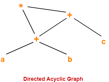
Example: ( a + b ) x ( a + b + c )

Three Address Code for the given expression is-

 T1 = a + b

T2 = T1 + c

T3 = T1 x T2

Now, Directed Acyclic Graph is-

 

 

From the constructed DAG, we observe-

• The common sub-expression (a+b) has been expressed into a single node in the DAG.
• The computation is carried out only once and stored in the identifier T1 and reused later.

This illustrates how the construction scheme of a DAG identifies the common sub-expression and helps in eliminating its re-computation later.

The Value-Number Method for Constructing DAG's 

• Often, the nodes of a syntax tree or DAG are stored in an array of records. 
• Each row of the array represents one record, and therefore one node. 
• In each record, the first field is an operation code, indicating the label of the node.

In Fig. 6.6(b), leaves have one additional field, which holds the lexical value (either a symbol-table pointer or a constant, in this case), and interior nodes have two additional fields indicating the left and right children. 

In this array, we refer to nodes by giving the integer index of the record
for that node within the array. This integer historically has been called the
value number for the node or for the expression represented by the node.

Algorithm 6.3: The value-number method for constructing the nodes of a DAG. 

 
INPUT: Label op , node l , and node r .
OUTPUT: The value number of a node in the array with signature h op ; l; r i .
METHOD: 

• Search the array for a node M with label op , left child l , and right child r . 
• If there is such a node, return the value number of M . 
• If not, create in the array a new node N with label op , left child l , and right child r , and return its value number.

While Algorithm 6.3 yields the desired output, searching the entire array
every time we are asked to locate one node is expensive, especially if the array
holds expressions from an entire program. 

A more efficient approach is to use a hash table, in which the nodes are put into "buckets", each of which typically will have only a few nodes. The hash table is one of several data structures that support dictionaries efficiently.  

A dictionary is an abstract data type that allows us to insert and delete elements of a set, and to determine whether a  given element is currently in the set. A good data structure for dictionaries, such as a hash table, performs each of these operations in time that is constant or close to constant, independent of the size of the set.

To construct a hash table for the nodes of a DAG, 

we need a hash function h that computes the index of the bucket for a signature h op ; l; r i , in a way that distributes the signatures across buckets, so that it is unlikely that any one bucket will get much more than a fair share of the nodes. The bucket index h ( op ; l; r ) is computed deterministically from op , l , and r , so that we may repeat the calculation and always get to the same bucket index for node h op ; l; r i .
 

The buckets can be implemented as linked lists, as in Fig. 6.7. An array,
indexed by hash value, holds the bucket headers , each of which points to the
first cell of a list. Within the linked list for a bucket, each cell holds the value
number of one of the nodes that hash to that bucket. That is, node h op ; l; r i
can be found on the list whose header is at index h ( op ; l; r ) of the array.