Mathematical Foundations

 1. Define vector space.Give example.

A vector space is a set V on which two operations + and · are defined, called vector addition and scalar multiplication.

The operation + (vector addition) must satisfy the following conditions:

Closure: If u and v are any vectors in V, then the sum   u + v   belongs to V.

(1) Commutative law: For all vectors u and v in V,     u + v = v + u

(2) Associative law: For all vectors u, v, w in V,     u + (v + w) = (u + v) + w

(3) Additive identity: The set V contains an additive identity element, denoted by 0, such that for any vector v in V,     0 + v = v   and   v + 0 = v.

(4) Additive inverses: For each vector v in V, the equations     v + x = 0   and   x + v = 0     have a solution x in V, called an additive inverse of v, and denoted by - v.

The operation · (scalar multiplication) is defined between real numbers (or scalars) and vectors, and must satisfy the following conditions:

Closure: If v in any vector in V, and c is any real number, then the product   c · v   belongs to V.

(5) Distributive law: For all real numbers c and all vectors u, v in V,     c · (u + v) = c · u + c · v

(6) Distributive law: For all real numbers c, d and all vectors v in V,     (c+d) · v = c · v + d · v

(7) Associative law: For all real numbers c,d and all vectors v in V,     c · (d · v) = (cd) · v

(8) Unitary law: For all vectors v in V,     1 · v = v

 

The simplest example of a vector space is the trivial one: {0}, which contains only the zero vector (see the third axiom in the Vector space article). Both vector addition and scalar multiplication are trivial. A basis for this vector space is the empty set, so that {0} is the 0-dimensional vector space over F.  

 

2. State and prove Bayes Theorem 

Bayes’ Theorem describes the probability of occurrence of an event related to any condition. It is also considered for the case of conditional probability.

Bayes Theorem Statement

Let E₁, E₂,…, E_n be a set of events associated with a sample space S, where all the events E₁, E₂,…, E_n have nonzero probability of occurrence and they form a partition of S. Let A be any event associated with S, then according to Bayes theorem,

P(Ei│A) = P(Ei)P(A│Ei)∑k=1nP(Ek)P(A|Ek)

for any k = 1, 2, 3, …., n

Bayes Theorem Proof

According to the conditional probability formula,

P(Ei│A) = P(Ei∩A)P(A) ⋯⋯⋯⋯⋯⋯⋯⋯(1)

Using the multiplication rule of probability,
P(Ei∩A) = P(Ei)P(A│Ei)⋯⋯⋯⋯⋯⋯⋯⋯(2)

Using total probability theorem,
P(A) = ∑k=1n P(Ek)P(A|Ek)⋯⋯⋯⋯⋯⋯⋯⋯⋯⋯⋯(3)

Putting the values from equations (2) and (3) in equation 1, we get

P(Ei│A) = P(Ei)P(A│Ei)∑k=1n P(Ek)P(A|Ek)

Note:

The following terminologies are also used when the Bayes theorem is applied:

Hypotheses: The events E₁, E₂,… E_n is called the hypotheses

Prior Probability: The probability P(E_i) is considered as the prior probability of hypothesis E_i

Posterior Probability: The probability P(E_i|A) is considered as the posterior probability of hypothesis E_i
Bayes’ theorem is also called the formula for the probability of “causes”. Since the E_i‘s are a partition of the sample space S, one and only one of the events E_i occurs (i.e. one of the events E_i must occur and the only one can occur). Hence, the above formula gives us the probability of a particular E_i (i.e. a “Cause”), given that the event A has occurred.

Bayes Theorem Formula

If A and B are two events, then the formula for Bayes theorem is given by:

P(A|B) = P(A∩B)/P(B)

Where P(A|B) is the probability of condition when event A is occurring while event B has already occurred.

P(A ∩ B) is the probability of event A and event B

P(B) is the probability of event B

3. State and prove Chapman- Kolmogorov Equations

Definition: The n-step transition probability that a process currently in state i will be in state j after n additional transitions.

By using the Markov property and the law of total probability, we realize that

 Pij(t+s)=r∑k=0Pik(t)Pkj(s)for all i,j∈ X,t,s>0 

These equations are known as the Chapman-Kolmogorov equations. The equations may be written in matrix terms as 

P(t+s)=P(t)·P(s) 

4. Derive Birth n Death Process 

The birth–death process (or birth-and-death process) is a special case of continuous-time Markov process where the state transitions are of only two types: "births", which increase the state variable by one and "deaths", which decrease the state by one. T

Birth–death processes have many applications in demography, queueing theory, performance engineering, epidemiology, biology and other areas.  

When a birth occurs, the process goes from state n to n + 1. When a death occurs, the process goes from state n to state n − 1. The process is specified by birth rates ${\displaystyle \{\lambda _{i}\}_{i=0\dots \infty }}$ and death rates ${\displaystyle \{\mu _{i}\}_{i=1\dots \infty }}$. 

5. State Pollaczek–Khinchine formula

The Pollaczek–Khinchine formula states a relationship between the queue length and service time distribution Laplace transforms for an M/G/1 queue (where jobs arrive according to a Poisson process and have general service time distribution). The term is also used to refer to the relationships between the mean queue length and mean waiting/service time in such a model.^[1] 

6. Define Markov Chain

A stochastic process has the Markov property if the conditional probability distribution of future states of the process (conditional on both past and present values) depends only upon the present state; that is, given the present, the future does not depend on the past. A process with this property is said to be Markovian or a Markov process. The most famous Markov process is a Markov chain. Brownian motion is another well-known Markov process.

Markov property refers to the memoryless property of a stochastic process. That is, (the probability of) future actions are not dependent upon the steps that led up to the present state.

A Markov chain is a stochastic model describing a sequence of possible events in which the probability of each event depends only on the state attained in the previous event.

Markov chains have many applications as statistical models of real-world processes, such as studying cruise control systems in motor vehicles, queues or lines of customers arriving at an airport, currency exchange rates and animal population dynamics.

 

Ergodicity

A state i is said to be ergodic if it is aperiodic and positive recurrent.

Queueing Theory

Queuing theory (or queueing theory) refers to the mathematical study of the formation, function, and congestion of waiting lines, or queues.

Queuing are the most frequently encountered problems in everyday life. 

For example, queue at a cafeteria, library, bank, etc. Common to all of these cases are the arrivals of objects requiring service and the attendant delays when the service mechanism is busy. 

Waiting lines cannot be eliminated completely, but suitable techniques can be used to reduce the waiting time of an object in the system. A long waiting line may result in loss of customers to an organization. 

Waiting time can be reduced by providing additional service facilities, but it may result in an increase in the idle time of the service mechanism. 

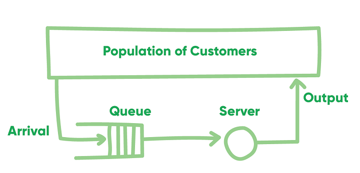
To illustrate, let’s take two examples. When looking at the queuing situation at a bank, the customers are people seeking to deposit or withdraw money, and the servers are the bank tellers. When looking at the queuing situation of a printer, the customers are the requests that have been sent to the printer, and the server is the printer.

 

Queuing theory uses the Kendall notation to classify the different types of queuing systems, or nodes. 

Queuing nodes are classified using the notation A/S/c/K/N/D where:

• A is the arrival process
• S is the mathematical distribution of the service time
• c is the number of servers
• K is the capacity of the queue, omitted if unlimited
• N is the number of possible customers, omitted if unlimited
• D is the queuing discipline, assumed first-in-first-out if omitted

The general form of a queuing model as,

(a/b/c): (d/e)

where,

• a is the arrival process or inter arrival time
• b is the mathematical distribution of the service time
• c is the number of servers
• d is the capacity of the queue, omitted if unlimited
• e is the queuing discipline, assumed first-in-first-out if omitted

For example, think of an ATM.

It can serve: one customer at a time; in a first-in-first-out order; with a randomly-distributed arrival process and service distribution time; unlimited queue capacity; and unlimited number of possible customers.

 Different types of Queuing Model

[(M/M/1):(∞/FIFO)]

[(M/M/s):(∞/FIFO)]

[(M/M/1):(k/FIFO)]

[(M/M/s):(k/FIFO)]

Operating characteristic of a Queuing System 

Queuing length(Lq) 

System length(LS)

Waiting time in queue (Wq) 

Waiting time in system(WS)

M/M/1 Model (Single Server Poisson Queue)

Queuing theory would describe this system as a M/M/1 queue (“M” here stands for Markovian, a statistical process to describe randomness).

This model is based on the following assumptions:

1. The arrivals follow Poisson distribution, with a mean arrival rate λ.
2. The service time has exponential distribution, average service rate μ.
3. Arrivals are infinite population α.
4. Customers are served on a First-in, First-out basis (FIFO).
5. There is only a single server. 

Single Server Queuing System Example

System of Steady-state Equations

In this method, the question arises whether the service can meet the customer demand. This depends on the values of λ and μ.

If λ ≥ m, i.e., if arrival rate is greater than or equal to the service rate, the waiting line would increase without limit. Therefore for a system to work, it is necessary that λ < μ.

 

• Traffic intensity ρ = λ / μ. This refers to the probability of time, the service station is busy

• Probability that the system is idle or there are no customers in the system

P0 = 1 – ρ.

• From this, the probability of having exactly one customer in the system is P1 = ρ P0.

• The probability of having exactly n customers in the system is

Pn = ρnP0 =(λ / μ)^n P0

Little’s Law connects the capacity of a queuing system, the average time spent in the system, and the average arrival rate into the system without knowing any other features of the queue. The formula is quite simple and is written as follows:

 or transformed to solve for the other two variables so that:

Where:

• L is the average number of customers in the system
• λ (lambda) is the average arrival rate into the system
• W is the average amount of time spent in the system

A line in a virtual waiting room

At Queue-it, we show visitors their wait time in the online queue using a calculation based on Little’s Law, adding in factors to account for no-shows and re-entries:

 Where:

• L is the number of users ahead in line
• λ (lambda) is rate of redirects to the website or app, in users per minute
• N is the no-show ratio
• R is the re-entry rate to the queue
• W is the estimated wait time, in minutes

Example 1: Arrivals at a telephone booth are considered to be Poisson distributed with an average time of 12 minutes between one arrival and the next. The length of phone call is assumed to be distributed exponentially, with mean 4 minutes.

(i) What is the probability that a person arriving at the booth will have to wait?
(ii) The telephone department will install a second booth when convinced that an arrival would expect waiting for at least 3 minutes for phone call. By how much should the flow of arrivals increase in order to justify a second booth?
(iii) What is the average length of the queue that forms from time to time?
(iv) What is the probability that it will take him more than 10 minutes altogether to wait for the phone and complete his call?

(v) Estimate the fraction of the phone will be in use. 

(vi) Find the avg. no. of persons waiting in the system.

Solution:  

Given λ= 1/12 = 0.08 person per minute.
μ = 1/4 = 0.25 person per minute.

(i) Probability that a person arriving at the booth will have to wait,
P (w > 0) = 1 – P₀
= 1 – (1 - λ / μ) = λ / μ
= 0.33

(ii) The installation of second booth will be justified if the arrival rate is more than the waiting time.
We have, W_q >=3 min

by the equation of W_q ,we will be finding λ by simplifying  _{Wq =3}

λ>=0.10

Hence the increase in arrival rate is, 0.10 arrivals per minute.

(iii) Average number of units in the system is given by,

L_s= ρ/1- ρ
= 0.3/1-0.3
= 0.43 customers

(iv) Probability of waiting for 10 minutes or more is given by,

P(W>10)= e^-( μ-λ)t

=e^-(0.25-0.08)10

=0.182

For More Problems 

Short Problems 

https://www.wisdomjobs.com/e-university/quantitative-techniques-for-management-tutorial-297/single-server-queuing-model-9934.html 

Linear Algebra: Rank of the Matrix (M1.3)

 Echelon form means that the matrix is in one of two states:

• Row echelon form.
• Reduced row echelon form

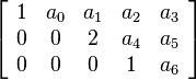
A matrix is in row echelon form if it meets the following requirements:

• The first non-zero number from the left (the “leading coefficient“) is always to the right of the first non-zero number in the row above.
• Rows consisting of all zeros are at the bottom of the matrix.

  

REF

https://www.statisticshowto.com/matrices-and-matrix-algebra/reduced-row-echelon-form-2/ 

Linear Algebra: Matrix Inverse (M1.2)

 

 

 

 

Linear Algebra: Matrix operations (M1.1)

Matrix operations mainly involve three algebraic operations which are addition of matrices, subtraction of matrices, and multiplication of matrices. Matrix is a rectangular array of numbers or expressions arranged in rows and columns.

As far as linear algebra is concerned, the two most important operations with vectors are vector addition [adding two (or more) vectors] and scalar multiplication (multiplying a vector by a scalar).

Operations

Addition, subtraction and multiplication are the basic operations on the matrix. To add or subtract matrices, these must be of identical order and for multiplication, the number of columns in the first matrix equals the number of rows in the second matrix.

• Addition of Matrices
• Subtraction of Matrices
• Scalar Multiplication of Matrices
• Multiplication of Matrices

Matrix Addition

If A[a_ij]_mxn and B[b_ij]_mxn are two matrices of the same order then their sum A + B is a matrix, and each element of that matrix is the sum of the corresponding elements. 

i.e. A + B = [a_ij + b_ij]_mxn

 For the Example:

Properties of Matrix Addition: If a, B and C are matrices of same order, then

(a) Commutative Law: A + B = B + A

(b) Associative Law:  (A + B) + C = A + (B + C)

(c) Identity of the Matrix: A + O =  O + A = A, where O is zero matrix which is additive identity of the matrix,

(d) Additive Inverse: A + (-A) = 0 = (-A) + A, where (-A) is obtained by changing the sign of every element of A which is additive inverse of the matrix,

(e) $\left. \begin{matrix} A+B=A+C \\ B+A=C+A \\ \end{matrix} \right\}\Rightarrow B=C$

(f) $tr\left( A\pm B \right)=tr\left( A \right)\pm tr\left( B \right)$

(g) If A + B = 0 = B + A, then B is called additive inverse of A and also A is called the additive inverse of A.

Subtraction of Matrices

If A and B are two matrices of the same order, then we define $A-B=A+\left( -B \right).$

We can subtract the matrices by subtracting each element of one matrix from the corresponding element of the second matrix. i.e. A – B = [a_ij – b_ij]_mxn

Scalar Multiplication of Matrices

If $A={{\left[ {{a}_{ij}} \right]}_{m\times n}}$ is a matrix and k any number, then the matrix which is obtained by multiplying the elements of A by k is called the scalar multiplication of A by k and it is denoted by k A thus if $A={{\left[ {{a}_{ij}} \right]}_{m\times n}}$

Then $k{{A}_{m\,\times n}}={{A}_{m\,\times \,n}}k=\left[ k{{a}_{i\times j}} \right]$

Properties of Scalar Multiplication: If A, B are matrices of the same order and λ and μ are any two scalars then;

(a) $\lambda \left( A+B \right)=\lambda A+\lambda B$

(b) $\left( \lambda +\mu \right)A=\lambda A+\mu A$

(c) $\lambda \left( \mu A \right)=\left( \lambda \,\mu A \right)=\mu \left( \lambda A \right)$

(d) $\left( -\lambda A \right)=-\left( \lambda A \right)=\lambda \left( -A \right)$

(e) $tr\left( kA \right)=k\,\,tr\,\,\left( A \right)$

 

Multiplication of Matrices

If A and B be any two matrices, then their product AB will be defined only when the number of columns in A is equal to the number of rows in B.

The first step in defining matrix multiplication is to recall the definition of the dot product of two vectors. Let r and c be two n‐vectors. Writing r as a 1 x n row matrix and c as an n x 1 column matrix, the dot product of r and c is

​

Note that in order for the dot product of r and c to be defined, both must contain the same number of entries. Also, the order in which these matrices are written in this product is important here: The row vector comes first, the column vector second. 

Properties of matrix multiplication

(a) Matrix multiplication is not commutative in general, i.e. in general $AB\ne BA.$

(b) Matrix multiplication is associative, i.e. (AB)C = A(BC).

(c) Matrix multiplication is distributive over matrix addition, i.e. A.(B + C) = A.B + A.C and (A + B)C = AC + BC.

(d) If A is an m × n matrix, then ${{I}_{m}}A=A=A{{I}_{n}}.$

(e) The product of two matrices can be a null matrix while neither of them is null, i.e. if AB = 0, it is not necessary that either A = 0 or B = 0.

(f) If A is an m × n matrix and O is a null matrix then ${{A}_{m\,\times n}}.{{O}_{n\,\times p}}={{O}_{m\,\times p}}.$ i.e. the product of the matrix with a null matrix is always a null matrix.

(g) If AB = 0 (It does not mean that A = 0 or B = 0, again the product of two non-zero matrices may be a zero matrix).

(h) If AB = AC , B ≠ C (Cancellation Law is not applicable).

(i) $tr\left( AB \right)=tr\left( BA \right).$

j) There exist a multiplicative identity for every square matrix such AI = IA = A

Matrix Transpose

If A is m × n, the transpose of A is the n × m matrix, denoted by A^T , whose columns are formed from the corresponding rows of A.

  

A square matrix has the same number of rows and columns. An identity matrix is a square matrix with ones on the diagonal from upper left to lower right and zeros elsewhere. For example:

   I = 
       1 0 0 
       0 1 0
       0 0 1

Such a matrix is often denoted I.

 

REF

https://www.cliffsnotes.com/study-guides/algebra/linear-algebra/matrix-algebra/operations-with-matrices 

https://byjus.com/jee/matrix-operations/