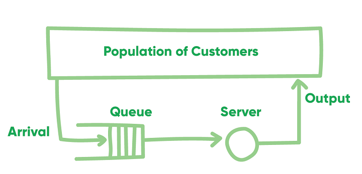
Queuing are the most frequently encountered problems in everyday life.
For example, queue at a cafeteria, library, bank, etc. Common to all of these cases are the arrivals of objects requiring service and the attendant delays when the service mechanism is busy.
Waiting lines cannot be eliminated completely, but suitable techniques can be used to reduce the waiting time of an object in the system. A long waiting line may result in loss of customers to an organization.
Waiting time can be reduced by providing additional service facilities, but it may result in an increase in the idle time of the service mechanism.
To illustrate, let’s take two examples. When looking at the queuing situation at a bank, the customers are people seeking to deposit or withdraw money, and the servers are the bank tellers. When looking at the queuing situation of a printer, the customers are the requests that have been sent to the printer, and the server is the printer.
Queuing theory uses the Kendall notation to classify the different types of queuing systems, or nodes.
Queuing nodes are classified using the notation A/S/c/K/N/D where:
- A is the arrival process
- S is the mathematical distribution of the service time
- c is the number of servers
- K is the capacity of the queue, omitted if unlimited
- N is the number of possible customers, omitted if unlimited
- D is the queuing discipline, assumed first-in-first-out if omitted
The general form of a queuing model as,
(a/b/c): (d/e)
where,
- a is the arrival process or inter arrival time
- b is the mathematical distribution of the service time
- c is the number of servers
- d is the capacity of the queue, omitted if unlimited
- e is the queuing discipline, assumed first-in-first-out if omitted
For example, think of an ATM.
It can serve: one customer at a time; in a first-in-first-out order; with a randomly-distributed arrival process and service distribution time; unlimited queue capacity; and unlimited number of possible customers.
Different types of Queuing Model
[(M/M/1):(∞/FIFO)]
[(M/M/s):(∞/FIFO)]
[(M/M/1):(k/FIFO)]
[(M/M/s):(k/FIFO)]
Operating characteristic of a Queuing System
Queuing length(Lq)
System length(LS)
Waiting time in queue (Wq)
Waiting time in system(WS)
M/M/1 Model (Single Server Poisson Queue)
Queuing theory would describe this system as a M/M/1 queue (“M” here stands for Markovian, a statistical process to describe randomness).
This model is based on the following assumptions:
- The arrivals follow Poisson distribution, with a mean arrival rate λ.
- The service time has exponential distribution, average service rate μ.
- Arrivals are infinite population α.
- Customers are served on a First-in, First-out basis (FIFO).
- There is only a single server.
Single Server Queuing System Example
System of Steady-state Equations
In this method, the question arises whether the service can meet the customer demand. This depends on the values of λ and μ.
If λ ≥ m, i.e., if arrival rate is greater than or equal to the service rate, the waiting line would increase without limit. Therefore for a system to work, it is necessary that λ < μ.
Traffic intensity ρ = λ / μ. This refers to the probability of time, the service station is busy
Probability that the system is idle or there are no customers in the system
P0 = 1 – ρ.
From this, the probability of having exactly one customer in the system is P1 = ρ P0.
The probability of having exactly n customers in the system is
Pn = ρnP0 =(λ / μ)^n P0


Little’s Law connects the capacity of a queuing system, the average
time spent in the system, and the average arrival rate into the system
without knowing any other features of the queue. The formula is quite
simple and is written as follows:
or transformed to solve for the other two variables so that:
Where:
- L is the average number of customers in the system
- λ (lambda) is the average arrival rate into the system
- W is the average amount of time spent in the system
A line in a virtual waiting room
At Queue-it, we show visitors their wait time in the online queue using a calculation based on Little’s Law, adding in factors to account for no-shows and re-entries:
Where:
- L is the number of users ahead in line
- λ (lambda) is rate of redirects to the website or app, in users per minute
- N is the no-show ratio
- R is the re-entry rate to the queue
- W is the estimated wait time, in minutes
Example 1: Arrivals at a telephone booth are considered to be Poisson distributed with an average time of 12 minutes between one arrival and the next. The length of phone call is assumed to be distributed exponentially, with mean 4 minutes.
(i) What is the probability that a person arriving at the booth will have to wait?
(ii) The telephone department will install a second booth when convinced
that an arrival would expect waiting for at least 3 minutes for phone
call. By how much should the flow of arrivals increase in order to
justify a second booth?
(iii) What is the average length of the queue that forms from time to time?
(iv) What is the probability that it will take him more than 10 minutes altogether to wait for the phone and complete his call?
(v) Estimate the fraction of the phone will be in use.
(vi) Find the avg. no. of persons waiting in the system.
Solution:
Given λ= 1/12 = 0.08 person per minute.
μ = 1/4 = 0.25 person per minute.
(i) Probability that a person arriving at the booth will have to wait,
P (w > 0) = 1 – P0
= 1 – (1 - λ / μ) = λ / μ
= 0.33
(ii) The installation of second booth will be justified if the arrival rate is more than the waiting time.
We have, Wq >=3 min
by the equation of Wq ,we will be finding λ by simplifying Wq =3
λ>=0.10
Hence the increase in arrival rate is, 0.10 arrivals per minute.
(iii) Average number of units in the system is given by,
Ls= ρ/1- ρ
= 0.3/1-0.3
= 0.43 customers
(iv) Probability of waiting for 10 minutes or more is given by,
P(W>10)= e^-( μ-λ)t
=e^-(0.25-0.08)10
=0.182
M/M/S case (Random Arrival, Random Service, and S service channel)
(Multiple Servers, Unlimited Queue Model)
(M/M/C) (∞/FCFS) Model

