Tuesday, October 26, 2021

Solutions to Compilers Second Edition Principles, Techniques, & Tools

 Chapter 5

 5.1.3 Exercises for Section 5.1

Exercise 5.1.1 : For the SDD of Fig. 5.1, give annotated parse trees for the

following expressions:

a) (3 + 4) * (5 + 6) n.


b) 1 * 2 * 3 * (4 + 5) n.


c) (9 + 8 * (7 + 6) + 5) * 4 n.


Exercise 5.1.2 : Extend the SDD of Fig. 5.4 to handle expressions as in Fig. 5.1.

1)L -> EnL.val = E.val
2)E -> TE'E'.inh = T.val
E.val = E'.syn
3)E' -> +TE_1'E_1'.inh = E'.inh + T.val
E'.syn = E_1'.syn
4)E' -> εE'.syn = E'.inh
5)T -> FT'T'.inh = F.val
T.val = T'.syn
6)T' -> *FT_1'T_1'.inh = T'.inh * F.val
T'.syn = T_1'.syn
7)T' -> εT'.syn = T'.inh
8)F -> (E)F.val = E.val
9)F -> digitF.val = digit.lexval

Exercise 5.1.3 : Repeat Exercise 5.1.1, using your SDD from Exercise 5.1.2.


Chapter 6

 Exercises for Section 6.1

Exercise 6.1.1 : Construct the DAG for the expression

((x + y) - ((x + y) * (x -y))) + ((x + y) * (x - y))


Exercise 6.1.2 : Construct the DAG and identify the value numbers for the subexpressions of the following expressions, assuming + associates from the left.

a) a + b + (a + b).

b) a + b + a + b.

c) a + a + 􀀀a + a + a + (a + a + a + a))

a)

1ida
2idb
3+12
4+33


b)


1ida
2idb
3+12
4+31
5+42


c)

1ida
2+11
3+21
4+31
5+34
6+25


6.2.5 Exercises for Section 6.2
Exercise 6.2.1 : Translate the arithmetic expression a + -(b + c) into:
a) A syntax tree.
b) Quadruples.
c) Triples.
d) Indirect triples.

a)

b)

oparg1arg2result
0+bct1
1minust1t2
2+at2t3

c)

oparg1arg2
0+bc
1minus(0)
2+a(1)
d)


instruction
0(0)
1(1)
2(2)

Exercise 6.2.2 : Repeat Exercise 6.2.1 for the following assignment statements:
i. a = b[i] + c[j].
ii. a[i] = b*c - b*d.
iii. x = f(y+1) + 2.
iv. x = *p + &y.

1
  0) =[]   b    i    t1
  1) =[]   c    j    t2
  2) +     t1   t2   t3
  3) =     t3        a  


  0) =[]   b    i
  1) =[]   c    j
  2) +     (0)  (1)
  3) =     a    (2)  


  Instructions
( 0) 
(1)
(2)
(3)

2
  0) *    b    c    t1
  1) *    b    d    t2
  2) -    t1   t2   t3
  3) []=  a    i    t4
  4) =    t3        t4

  0) *    b    c
  1) *    b    d
  2) -    (0)  (1)
  3) []=  a    i
  4) =    (3)  (2)

  
  0)
  1)
  2)
  3)
  4)

3
  0) +        y    1    t1
  1) param    t1
  2) call     f    1    t2
  3) +        t2    2   t3
  4) =        t3        x

  0) +        y     1
  1) param    (0)
  2) call     f     1
  3) +        (2)   2
  4) =        x     (3)


  0)
  1)
  2)
  3)
  4)


Exercise 6.2.3 : Show how to transform a three-address code sequence into one in which each de ned variable gets a unique variable name.

3adddress code sequence can be transformed into SSA in which each defines variable gets a unique variable name.
Static single-assignment form (SSA) is an intermediate representation that facilitates certain code optimizations. The all assignments in SSA are to variables with distinct names; hence the term static single-assignment.

6.3.7 Exercises for Section 6.3
Exercise 6.3.1 : Determine the types and relative addresses for the identifers in the following sequence of declarations:

float x;
record { float x; float y; } p;
record { int tag; float x; float y; } q;


S ->                  {top = new Evn(); offset = 0;}
     D 
D -> T id;            {top.put(id.lexeme, T.type, offset);
                       offset += T.width}
     D1
D -> ε
T -> int              {T.type = interget; T.width = 4;}
T -> float            {T.type = float; T.width = 8;}
T -> record '{'
                      {Evn.push(top), top = new Evn();
                       Stack.push(offset), offset = 0;}
     D '}'            {T.type = record(top); T.width = offset;
                       top = Evn.top(); offset = Stack.pop();}


line id      type        offset   Evn

  1) x       float       0        1

  2) x       float       0        2
  2) y       float       8        2
  2) p       record()    8        1

  3) tag     int         0        3
  3) x       float       4        3
  3) y       float       12       3
  3) q       record()    24       1     

Exercise 6.3.2 : Extend the handling of eld names in Fig. 6.18 to classes and single-inheritance class hierarchies.
a) Give an implementation of class Env that allows linked symbol tables, so that a subclass can either rede ne a eld name or refer directly to a eld name in a superclass.
b) Give a translation scheme that allocates a contiguous data area for the elds in a class, including inherited elds. Inherited elds must maintain the relative addresses they were assigned in the layout for the superclass.

6.4.5 Exercises for Section 6.4
Exercise 6.4.1 : Add to the translation of Fig. 6.19 rules for the following productions:
a) E ! E1  E2.
b) E ! + E1 (unary plus).

a)

E -> E1 * E2     { E.addr = new Temp();
                         E.code = E1.code || E2.code ||
                            gen(E.addr '=' E1.addr '*' E2.addr); }
                         
   | +E1             { E.addr = E1.addr;
                        E.code = E1.code; }


Exercise 6.4.2 : Repeat Exercise 6.4.1 for the incremental translation of Fig. 6.20.


E -> E1 * E2    { E.addr =  new Temp();
                         gen(E.addr '=' E1.addr '*' E2.addr; }
                         
   | +E1            { E.addr = E1.addr; }


Exercise 6.4.3 : Use the translation of Fig. 6.22 to translate the following
assignments:
a) x = a[i] + b[j].
b) x = a[i][j] + b[i][j].
! c) x = a[b[i][j]][c[k]].

a)


 t_1 = i * awidth
 t_2 = a[t_1]
 t_3 = j * bwidth
 t_4 = b[t_3]
 t_5 = t_2 + t_4
 x = t_5


b)

 t_1 = i * ai_width
 t_2 = j * aj_width
 t_3 = t_1 + t_2
 t_4 = a[t_3]
 t_5 = i * bi_width
 t_6 = j * bj_width
 t_7 = t_5 + t_6
 t_8 = b[t_7]
 t_9 = t_4 + t_8
 x = t_9


Exercise 6.4.4 : Revise the translation of Fig. 6.22 for array references of the
Fortran style, that is, id[E1; E2; : : : ; En] for an n-dimensional array.

a.type = array(i, array(j, w))
a.type.length = i
a.type.elem = array(j, w)


Exercise 6.4.5 : Generalize formula (6.7) to multidimensional arrays, and indicate what values can be stored in the symbol table and used to compute o sets. Consider the following cases:
a) An array A of two dimensions, in row-major form. The rst dimension has indexes running from l1 to h1, and the second dimension has indexes from l2 to h2. The width of a single array element is w.

3. A[i_1]]…[i_k] = base + 
                   (
                       (i_1 - l_1) * n_2 * … * n_k +
                       … + 
                       (i_k-1 - l_k-1) * n_k +
                       (i_k - l_k)
                   ) * w
                 
4. A[i_1]]…[i_k] = base + 
                   (
                       (i_1 - l_1) +
                       (i_2 - l_2) * n_1 + 
                       … +
                       (i_k - l_k) * n_k-1 * n_k-2 * … * n_1
                   ) * w

Code Generation || Issues in the Design of a Code Generator

  • The final phase in our compiler model is the code generator. 
  • It takes as input the intermediate representation (IR) produced by the front end of the compiler, along with relevant symbol table information, and produces as output a semantically equivalent target program
  • Compilers that need to produce efficient target programs, include an optimization phase prior to code generation. The optimizer maps the IR into IR from which more efficient code can be generated. In general, the code optimization and code-generation phases of a compiler, often referred to as the back end , may make multiple passes over the IR before generating the target program.

Code Generation 

A code generator has three primary tasks: 

  • Instruction selection involves choosing appropriate target-machine instructions to implement the IR statements. 
  • Register allocation and assignment involves deciding what values to keep in which registers. 
  • Instruction ordering involves deciding in what order to schedule the execution of instructions.

Issues in the Design of a Code Generator 

The most important criterion for a code generator is that it produce correct code. Correctness takes on special significance because of the number of special cases that a code generator might face. Given the premium on correctness, designing a code generator so it can be easily implemented, tested, and maintained is an important design goal.

1. Input to the Code Generator

  • The input to the code generator is the intermediate representation of the source program produced by the front end, along with information in the symbol table that is used to determine the run-time addresses of the data objects denoted by the names in the IR. 
  • The many choices for the IR include three-address representations such as quadruples, triples, indirect triples; virtual machine representations such as byte-codes and stack-machine code; linear representations such as post x notation; and graphical representations such as syntax trees and DAG's. 
  • We assume that the front end has scanned, parsed, and translated the source program into a relatively low-level IR, so that the values of the names appearing in the IR can be represented by quantities that the target machine can directly manipulate, such as integers and floating-point numbers. 
  • We also assume that all syntactic and static semantic errors have been detected, that the necessary type checking has taken place, and that type- conversion operators have been inserted wherever necessary. The code generator can therefore proceed on the assumption that its input is free of these kinds of errors.

 2. The Target Program

  • The instruction-set architecture of the target machine has a significant impact on the diffculty of constructing a good code generator that produces high-quality machine code. The most common target-machine architectures are RISC (reduced instruction set computer), CISC (complex instruction set computer), and stack based. 
  • A RISC machine typically has many registers, three-address instructions, simple addressing modes, and a relatively simple instruction-set architecture.  
  • In contrast, a CISC machine typically has few registers, two-address instructions, a variety of addressing modes, several register classes, variable-length instructions, and instructions with side effects.  
  • In a stack-based machine, operations are done by pushing operands onto a stack and then performing the operations on the operands at the top of the stack. To achieve high performance the top of the stack is typically kept in registers.


The target program is the output of the code generator.

  • Producing an absolute machine-language program as output has the advantage that it can be placed in a fixed location in memory and immediately executed. Programs can be compiled and executed quickly. 
  • Producing a relocatable machine-language program (often called an object module ) as output allows subprograms to be compiled separately. A set of relocatable object modules can be linked together and loaded for execution by a linking loader.
  • Producing an assembly-language program as output makes the process of code generation somewhat easier. We can generate symbolic instructions and use the macro facilities of the assembler to help generate code. The price paid is the assembly step after code generation.

3. Instruction Selection

  • The code generator must map the IR program into a code sequence that can be executed by the target machine. 
  • The complexity of performing this mapping is determined by factors such as the level of the IR the nature of the instruction-set architecture  the desired quality of the generated code.  
  • If the IR is high level, the code generator may translate each IR statement into a sequence of machine instructions using code templates. Such statement- by-statement code generation, however, often produces poor code that needs further optimization. 
  • If the IR reflects some of the low-level details of the underlying machine, then the code generator can use this information to generate more ecient code sequences.  
  • The nature of the instruction set of the target machine has a strong effect on the diculty of instruction selection. For example, the uniformity and completeness of the instruction set are important factors. 
  • Instruction speeds and machine idioms are other important factors. 
  • If we do not care about the efficiency of the target program, instruction selection is straightforward. For each type of three-address statement, we can design a code skeleton that defnes the target code to be generated for that construct. 

For example, every three-address statement of the form x = y + z , where x , y , and z are statically allocated, can be translated into the code sequence 

Here, the fourth statement is redundant since it loads a value that has just been stored, and so is the third if a is not subsequently used. The quality of the generated code is usually determined by its speed and
size.

4. Register Allocation

  • A key problem in code generation is deciding what values to hold in what registers. 
  • Registers are the fastest computational unit on the target machine, but we usually do not have enough of them to hold all values. Values not held in registers need to reside in memory.

The use of registers is often subdivided into two sub problems:
1. Register allocation , during which we select the set of variables that will reside in registers at each point in the program.
2. Register assignment , during which we pick the specific register that a variable will reside in.
 

Finding an optimal assignment of registers to variables is diffcult, even with single-register machines. Mathematically, the problem is NP-complete. The problem is further complicated because the hardware and/or the operating system of the target machine may require that certain register-usage conventions be observed.

Example: Certain machines require register-pairs (an even and next odd- numbered register) for some operands and results. For example, on some machines, integer multiplication and integer division involve register pairs. 

  • The multiplication instruction is of the form M x, y

where x , the multiplicand, is the odd register of an even/odd register pair and y , the multiplier, can be anywhere. The product occupies the entire even/odd register pair. 

  • The division instruction is of the form D x, y

where the dividend occupies an even/odd register pair whose even register is x ; the divisor is y . After division, the even register holds the remainder and the odd register the quotient.

5. Evaluation Order

  • The order in which computations are performed can a effect the effciency of the target code. 
  • Some computation orders require fewer registers to hold intermediate results than others. 
  • However, picking a best order in the general case is a dicult NP-complete problem.


Thursday, September 16, 2021

Particle swarm optimization (PSO)

  • Developed in 1995 by James Kennedy and Russ Eberhart.  
  • It was inspired by social behavior of bird flocking or fish schooling. 
  • PSO applies the concept of social interaction to problem solving. 
  • PSO is a computational method that optimizes a problem by iteratively trying to improve a candidate solution with regard to a given measure of quality.
  • PSO is a metaheuristic as it makes few or no assumptions about the problem being optimized and can search very large spaces of candidate solutions. 
  • Also, PSO does not use the gradient of the problem being optimized, which means PSO does not require that the optimization problem be differentiable as is required by classic optimization methods such as gradient descent and quasi-newton methods. 
  • However, metaheuristics such as PSO do not guarantee an optimal solution is ever found. 
  • PSO is a robust optimization technique that applies the social intelligence of swarms to solve optimization problems. 
  • Bird flocking and fish schooling are the example of swarm intelligence. In bird flocking, each swarm update its position by following collective intelligence of the group and its own intelligence. 
  • First version of this algorithm was proposed by J. Kennedy, R. Eberhart.In this version, a set of potential solutions (called as particles), are dispersed at various points in the solution space. Each point has some objective function value, and thus has fitness, for its current location. Each particle’s movement is influenced by the following two factors:
  1. The best fitness achieved by the particle so far. (BFS)
  2. The best fitness achieved by any particle in the neighbourhood.  (BFN)
Suppose that if the search space is n-dimensional, and then the particle i of the swarm can be represented by an n-dimensional vector Xi= (xi1, xi2, …,xin). The velocity of this particle can be represented by another n-dimensional vector Vi= (vi1, vi2, …, vin). 

The fitness of each particle can be evaluated according to the objective function of optimization problem. The best previously visited position of the particle i is noted as its individual best position Pi= (pi1,pi2,…,pin). 

The position of the best individual of the whole swarm is noted as the global best position G= (g1,g2, …,gn). At each step, the velocity of particle and its new position will be assigned according to the following two equations:
Vi=ω∗Vi+c1∗r1∗(Pi Xi)+c2∗r2∗(GXi)                                                              (1)
Xi=Xi+Vi                                                                                                              (2) 
 
Where, ω is called the inertia weight that controls the impact of previous velocity of particle on its current one. r1, r2 are independently uniformly distributed random variables with range (0, 1). c1, c2 are positive constant parameters called acceleration coefficients which control the maximum step size. 

In PSO, Eq. (1) is used to calculate the new velocity according to its previous velocity and to the distance of its current position from both its own best historical position and the best position of the entire population or its neighbourhood. Generally, the value of each component in V can be clamped to the range [-vmax, vmax] to control excessive roaming of particles outside the search space. Then the particle flies toward a new position according Eq. (2). This process is repeated until a user-defined stopping criterion is reached.

 #Bird Flocking

A flock is a gathering of a group of same species animals in order to forage or travel with one another. In avians flocks are typically seen in association with migration. While this is true it can also be seen that flocking is important in safety from predation and foraging benefits.

Flocking is the behavior exhibited when a group of birds, called a flock, are foraging or in flight.

From the perspective of the mathematical modeller, "flocking" is the collective motion by a group of self-propelled entities and is a collective animal behavior exhibited by many living beings such as birdsfishbacteria, and insects. It is considered an emergent behavior arising from simple rules that are followed by individuals and does not involve any central coordination.

In 1986, Craig Reynolds described this process in 3 simple behaviors:

  • Separation- avoid crowding local flockmates
  • Alignment- move towards the average heading of local flockmates
  • Cohesion- move toward the average position of local flockmates

#Fish Schooling

A school is a group of fish swimming in a synchronizing and polarized way. The individuals of this group adopt a schooling behavior (Pitcher, 1983). Schooling behaviors are characterized by the tendency to polarize, with individuals adopting the same orientation and swimming in the same direction

Fish schooling and aggregation behaviors are some of the most prominent social and group activities exhibited by fishes.

• Fish may school or form aggregations for many reasons, including foraging, reproduction, and defense from predators.

•One of the most enduring hypotheses regarding fish schooling is that fish in schools can obtain a hydrodynamic advantage, thus reducing the cost of locomotion, by taking advantage of the wakes shed by neighbors within the school.

Terminologies in PSO

•Collection of flying particles (swarm) - Changing solutions

• Search area - Possible solutions

•Movement towards a promising area to get the global optimum

•Each particle keeps track:
its best solution, personal best, pbest or lbest
the best value of any particle, global best, gbest 

  • Each particle keeps track of its coordinates in the solution space which are associated with the best solution (fitness) that has achieved so far by that particle. This value is called personal best , pbest. 
  • Another best value that is tracked by the PSO is the best value obtained so far by any particle in the neighborhood of that particle. This value is called gbest. 
  • The basic concept of PSO lies in accelerating each particle toward its pbest and the gbest locations, with a random weighted accelaration at each time step.

Working 

It solves a problem by having a population of candidate solutions, here dubbed particles, and moving these particles around in the search-space according to simple mathematical formula over the particle's position and velocity. 

Each particle's movement is influenced by its local best known position, but is also guided toward the best known positions in the search-space, which are updated as better positions are found by other particles. This is expected to move the swarm toward the best solutions. 
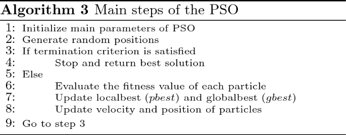

Human action recognition with deep learning and structural optimization  using a hybrid heuristic algorithm | SpringerLink 

The Particle Swarm Optimization (PSO) algorithm. | Download Scientific  Diagram

Particles Velocity
1. Inertia:
Makes the particle move in the same direction and with the same velocity
2. Personal Influence:
Improves the individual, Makes the particle return to a previous
position, better than the current, Conservative

3.
Social Influence: Makes the particle follow the best neighbors direction 

Intensification: explores the previous solutions, finds the best solution of a given region
Diversification: searches new solutions, finds the regions with potentially the best solutions

Evolution

PSO is originally attributed to Kennedy, Eberhart and Shi and was first intended for simulating social behaviour, as a stylized representation of the movement of organisms in a bird flock or fish school. The algorithm was simplified and it was observed to be performing optimization. The book by Kennedy and Eberhart describes many philosophical aspects of PSO and swarm intelligence. An extensive survey of PSO applications is made by Poli. Recently, a comprehensive review on theoretical and experimental works on PSO has been published by Bonyadi and Michalewicz.

The basic PSO parameters are swarm size or number of

particles, number of iterations, velocity components, and acceleration coefficients

illustrated bellow. In addition, PSO is also influenced by inertia weight, velocity

clamping, and velocity constriction

Neighborhood Topologies

A neighborhood must be defined for each particle [7]. This neighborhood

determines the extent of social interaction within the swarm and influences a

particular particle’s movement. Less interaction occurs when the neighborhoods in

the swarm are small [4]. For small neighborhood, the convergence will be slower

but it may improve the quality of solutions. For larger neighborhood, the

convergence will be faster but the risk that sometimes convergence occurs earlier

[7]. To solve this problem, the search process starts with small neighborhoods size

and then the small neighborhoods size is increased over time. This technique

ensures an initially high diversity with faster convergence as the particles move

towards a promising search region [4].

The PSO algorithm is social interaction among the particles in the entire swarm.

Particles communicate with one another by exchanging information about the

success of each particle in the swarm. When a particle in the whole swarm finds a

better position, all particles move towards this particle. This performance of the

particles is determined by the particles’ neighborhood [4]. Researchers have

worked on developing this performance by designing different types of

neighborhood structures [15]. Some neighborhood structures or topologies are

discussed below:


Figure 3.5 (a) illustrates the star topology, where each particle connects with every
other particle. This topology leads to faster convergence than other topologies, but
there is a susceptibility to be trapped in local minima. Because all particles know
each other, this topology is referred to as the gbest PSO.
Figure 3.5 (b) illustrates the ring topology, where each particle is connected only
with its immediate neighbors. In this process, when one particle finds a better
result, this particle passes it to its immediate neighbors, and these two immediate
neighbors pass it to their immediate neighbors, until it reaches the last particle.
Thus the best result found is spread very slowly around the ring by all particles.
Convergence is slower, but larger parts of the search space are covered than with
the star topology. It is referred as the lbest PSO.
Figure 3.5 (c) illustrates the wheel topology, in which only one particle (a focal
particle) connects to the others, and all information is communicated through this
particle. This focal particle compares the best performance of all particles in the
swarm, and adjusts its position towards the best performance particle. Then the
new position of the focal particle is informed to all the particles.
Figure 3.5 (d) illustrates a four clusters topology, where four clusters (or cliques)
are connected with two edges between neighboring clusters and one edge between
opposite clusters.
There are more different neighborhood structures or topologies (for instance,
pyramid topology, the Von Neumann topology and so on), but there is no the best
topology known to find the optimum for all kinds of optimization problems.

Neighbourhoods and topologies

  • The topology of the swarm defines the subset of particles with which each particle can exchange information. 
  • The basic version of the algorithm uses the global topology as the swarm communication structure. This topology allows all particles to communicate with all the other particles, thus the whole swarm share the same best position g from a single particle. However, this approach might lead the swarm to be trapped into a local minimum, thus different topologies have been used to control the flow of information among particles. 
  • For instance, in local topologies, particles only share information with a subset of particles. This subset can be a geometrical one – for example "the m nearest particles" – or, more often, a social one, i.e. a set of particles that is not depending on any distance. 
  • In such cases, the PSO variant is said to be local best (vs global best for the basic PSO).

A commonly used swarm topology is the ring, in which each particle has just two neighbours, but there are many others. The topology is not necessarily static. In fact, since the topology is related to the diversity of communication of the particles, some efforts have been done to create adaptive topologies (SPSO,  APSO,  stochastic star, TRIBES, Cyber Swarm, and C-PSO).

 Inshort,

Two different kinds of neighborhoods are defined for PSO:

1. In the gbest swarm, all the particles are neighbors of each other; thus, the position of the best overall particle in the swarm is used in the social term of the velocity update equation.

•It is assumed that gbest swarms converge fast, as all the particles are attracted simultaneously to the best part of the search space.

•However, if the global optimum is not close to the best particle, it may be impossible to the swarm to explore other areas; this means that the swarm can be trapped in local optima.

2. In the pbest / lbest swarm, only a specific number of particles (neighbor count) can affect the velocity of a given particle.

•The swarm will converge slower but can locate the global optimum with a greater chance. 

In the lbest / pbest topology, a number of neighbors are selected from each side of the particle

Convergence

In relation to PSO the word convergence typically refers to two different definitions:

  • Convergence of the sequence of solutions (aka, stability analysis, converging) in which all particles have converged to a point in the search-space, which may or may not be the optimum,
  • Convergence to a local optimum where all personal bests p or, alternatively, the swarm's best known position g, approaches a local optimum of the problem, regardless of how the swarm behaves.

Convergence of the sequence of solutions has been investigated for PSO.[15][16][17] These analyses have resulted in guidelines for selecting PSO parameters that are believed to cause convergence to a point and prevent divergence of the swarm's particles (particles do not move unboundedly and will converge to somewhere). However, the analyses were criticized by Pedersen[22] for being oversimplified as they assume the swarm has only one particle, that it does not use stochastic variables and that the points of attraction, that is, the particle's best known position p and the swarm's best known position g, remain constant throughout the optimization process. However, it was shown[38] that these simplifications do not affect the boundaries found by these studies for parameter where the swarm is convergent. Considerable effort has been made in recent years to weaken the modelling assumption utilized during the stability analysis of PSO,[39] with the most recent generalized result applying to numerous PSO variants and utilized what was shown to be the minimal necessary modeling assumptions.[40]

Convergence to a local optimum has been analyzed for PSO in[41] and.[42] It has been proven that PSO needs some modification to guarantee finding a local optimum.

This means that determining convergence capabilities of different PSO algorithms and parameters still depends on empirical results. One attempt at addressing this issue is the development of an "orthogonal learning" strategy for an improved use of the information already existing in the relationship between p and g, so as to form a leading converging exemplar and to be effective with any PSO topology. The aims are to improve the performance of PSO overall, including faster global convergence, higher solution quality, and stronger robustness.[43] However, such studies do not provide theoretical evidence to actually prove their claims. 

Comparison with other evolutionary computation techniques

• Unlike in genetic algorithms, evolutionary programming and evolutionary strategies, in PSO, there is no selection operation.

• All particles in PSO are kept as members of the population through the course of the run

• PSO is the only algorithm that does not implement the survival of the fittest.

• No crossover operation in PSO.

• eq 1resembles mutation in EP.

• In EP balance between the global and local search can be adjusted through the strategy parameter while in PSO the balance is achieved through the inertial weight factor (w) of eq. 1

Advantages & Disadvantages of PSO

Advantages of the PSO algorithm [14] [15]:

1) PSO algorithm is a derivative-free algorithm.

2) It is easy to implementation, so it can be applied both in scientific research

and engineering problems.

3) It has a limited number of parameters and the impact of parameters to the

solutions is small compared to other optimization techniques.

4) The calculation in PSO algorithm is very simple.

5) There are some techniques which ensure convergence and the optimum

value of the problem calculates easily within a short time.

6) PSO is less dependent of a set of initial points than other optimization

techniques.

7) It is conceptually very simple.

Disadvantages of the PSO algorithm [13]:

1) PSO algorithm suffers from the partial optimism, which degrades the

regulation of its speed and direction.

2) Problems with non-coordinate system (for instance, in the energy field)

exit.

Advantages
• Insensitive to scaling of design variables
• Simple implementation
• Easily parallelized for concurrent processing
• Derivative free
• Very few algorithm parameters
• Very efficient global search algorithm
 

 Disadvantages
• Tendency to a fast and premature convergence in mid optimum points
• Slow convergence in refined search stage (weak local search ability)

https://slideplayer.com/amp/1528196/

Millonas proposed five basic principles (van den Bergh 2001):

(1) Proximity: the swarm should be able to carry out simple space and time computations.

(2) Quality: the swarm should be able to sense the quality change in the environment and response it.

(3) Diverse response: the swarm should not limit its way to get the resources in a narrow scope.

(4) Stability: the swarm should not change its behavior mode with every environmental change.

(5) Adaptability: the swarm should change its behavior mode when this change is worthy.

Explain proximity principle, stability principle and adaptability principle of swam intelligence.

Proximity principle: The basic units of a swarm should be capable of giving the respond back to to environmental variance triggered by interactions among agents. However, some fundamental behaviors are shared such as living-resource searching and nest-building.

Principle of stability: The population should not change its mode of behavior every time the environment changes.

Principle of adaptability: The swarm is sensitive to the changes in the environment that result in different swarm behaviour.

https://www.techferry.com/articles/swarm-intelligence.html