Hashing (M3.3)

In a huge database structure, it is very inefficient to search all the index values and reach the desired data. Hashing technique is used to calculate the direct location of a data record on the disk without using index structure.

In this technique, data is stored at the data blocks whose address is generated by using the hashing function. The memory location where these records are stored is known as data bucket or data blocks. 

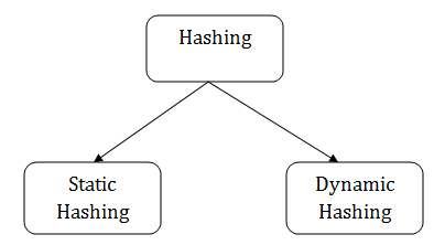
Hashing-

Hash Table- A hash table is a data structure for storing a set of items, so that we can quickly determine whether an
item is or is not in the set.

Hash Function- maps every possible item x to  a small integer h(x). Then we store x in slot h(x) in an array. The array is the hash table.

Let’s be a little more specific. We want to store a set of n items. Each item is an element of some finite 1 set U called the universe; we use u to denote the size of the universe, which is just the number of items in U . A hash table is an array T [1 .. m], where m is another positive integer, which we call the table size. Typically, m is much smaller than u. A hash function is any function of the form h: U → {0, 1, . . . , m − 1}, mapping each possible item in U to a slot in the hash table. We say that an item x hashes to the slot T [h(x)].

Limitations of Static hashing 

When the table is to be full, overflows increase. As overflows increase, the overall performance decreases. –We cannot just copy entries from smaller into a corresponding buckets of a bigger table. Allow the size of dictionary to grow and shrink. –The size of hash table can be changed dynamically.  

Dynamic Hashing

• The dynamic hashing method is used to overcome the problems of static hashing like bucket overflow.
• In this method, data buckets grow or shrink as the records increases or decreases. This method is also known as Extendable hashing method.
• This method makes hashing dynamic, i.e., it allows insertion or deletion without resulting in poor performance.

How to search a key

• First, calculate the hash address of the key.
• Check how many bits are used in the directory, and these bits are called as i.
• Take the least significant i bits of the hash address. This gives an index of the directory.
• Now using the index, go to the directory and find bucket address where the record might be.

How to insert a new record

• Firstly, you have to follow the same procedure for retrieval, ending up in some bucket.
• If there is still space in that bucket, then place the record in it.
• If the bucket is full, then we will split the bucket and redistribute the records.
  

To achieve a good hashing mechanism, It is important to have a good hash function with the following basic requirements:

1. Easy to compute: It should be easy to compute and must not become an algorithm in itself.

2. Uniform distribution: It should provide a uniform distribution across the hash table and should not result in clustering.

3. Less collisions: Collisions occur when pairs of elements are mapped to the same hash value. These should be avoided.

   Note: Irrespective of how good a hash function is, collisions are bound to occur. Therefore, to maintain the performance of a hash table, it is important to manage collisions through various collision resolution techniques.

For example:

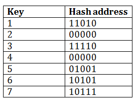
Consider the following grouping of keys into buckets, depending on the prefix of their hash address:

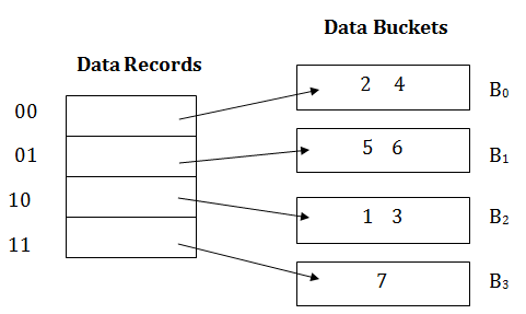
The last two bits of 2 and 4 are 00. So it will go into bucket B0. The last two bits of 5 and 6 are 01, so it will go into bucket B1. The last two bits of 1 and 3 are 10, so it will go into bucket B2. The last two bits of 7 are 11, so it will go into B3.

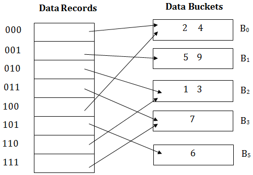
Insert key 9 with hash address 10001 into the above structure:

• Since key 9 has hash address 10001, it must go into the first bucket. But bucket B1 is full, so it will get split.
• The splitting will separate 5, 9 from 6 since last three bits of 5, 9 are 001, so it will go into bucket B1, and the last three bits of 6 are 101, so it will go into bucket B5.
• Keys 2 and 4 are still in B0. The record in B0 pointed by the 000 and 100 entry because last two bits of both the entry are 00.
• Keys 1 and 3 are still in B2. The record in B2 pointed by the 010 and 110 entry because last two bits of both the entry are 10.
• Key 7 are still in B3. The record in B3 pointed by the 111 and 011 entry because last two bits of both the entry are 11.

Advantages of dynamic hashing

• In this method, the performance does not decrease as the data grows in the system. It simply increases the size of memory to accommodate the data.
• In this method, memory is well utilized as it grows and shrinks with the data. There will not be any unused memory lying.
• This method is good for the dynamic database where data grows and shrinks frequently.

Disadvantages of dynamic hashing

• In this method, if the data size increases then the bucket size is also increased. These addresses of data will be maintained in the bucket address table. This is because the data address will keep changing as buckets grow and shrink. If there is a huge increase in data, maintaining the bucket address table becomes tedious.
• In this case, the bucket overflow situation will also occur. But it might take little time to reach this situation than static hashing.

UNIVERSAL HASHING

• Universal hashing (in a randomized algorithm or data structure) refers to selecting a hash function at random from a family of hash functions with a certain mathematical property. 
• This guarantees a low number of collisions in expectation, even if the data is chosen by an adversary. 
• Many universal families are known (for hashing integers, vectors, strings), and their evaluation is often very efficient. 
• Universal hashing has numerous uses in computer science, for example in implementations of hash tables, randomized algorithms, and cryptography.
  

https://www.javatpoint.com/dbms-hashing

Skip List (M3.1)

•  A skip list is a probabilistic data structure. 
• The skip list is used to store a sorted list of elements or data with a linked list. 
• It allows the process of the elements or data to view efficiently. 
• In one single step, it skips several elements of the entire list, which is why it is known as a skip list.
• The skip list is an extended version of the linked list. 
• It allows the user to search, remove, and insert the element very quickly. 
• It consists of a base list that includes a set of elements which maintains the link hierarchy of the subsequent elements.

A skip list starts with a basic, ordered, linked list. This list is sorted, but we can't do a binary search on it because it is a linked list and we cannot index into it.

Then, another layer is added on top of the bottom list. This new layer will include any given element from the previous layer with probability $p\mathrm{}$ This probability can vary, but oftentimes $\frac12$ is used. Additionally, the first node in the linked list is often always kept, as a header for the new layer.

Properties

• It has a height of $h$ which is the number of linked lists in it. It has a number of distinct elements, $n.$ And it has a probability $p,$ which is usually $\frac12.$
• $$The highest element (one that appears in the most lists) will appear in $\log_\frac{1}{p}(n)$ lists, on average, This, if we use $p = \frac12$, there are $\log_2(n)$ lists. This is the average value of $h$. Another way of saying "Every element in a linked list is in the linked list below it" is "Every element in level $S_{i+1}$ exists in level $S_i.$"
• Each element in the skip list has four pointers. It points to the node to its left, its right, its top, and its bottom. These quad-nodes will allow us to efficiently search through the skip list.

Skip List Basic Operations

There are the following types of operations in the skip list.

• Insertion operation: It is used to add a new node to a particular location in a specific situation.
• Deletion operation: It is used to delete a node in a specific situation.
• Search Operation: The search operation is used to search a particular node in a skip list.

Advantages of the Skip list

1. If you want to insert a new node in the skip list, then it will insert the node very fast because there are no rotations in the skip list.
2. The skip list is simple to implement as compared to the hash table and the binary search tree.
3. It is very simple to find a node in the list because it stores the nodes in sorted form.
4. The skip list algorithm can be modified very easily in a more specific structure, such as indexable skip lists, trees, or priority queues.
5. The skip list is a robust and reliable list.

Disadvantages of the Skip list

1. It requires more memory than the balanced tree.
2. Reverse searching is not allowed.
3. The skip list searches the node much slower than the linked list.

Applications of the Skip list

1. It is used in distributed applications, and it represents the pointers and system in the distributed applications.
2. It is used to implement a dynamic elastic concurrent queue with low lock contention.
3. It is also used with the QMap template class.
4. The indexing of the skip list is used in running median problems.
5. The skip list is used for the delta-encoding posting in the Lucene search.

---

Linear Algebra: Rank of the Matrix (M1.3)

 Echelon form means that the matrix is in one of two states:

• Row echelon form.
• Reduced row echelon form

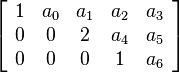
A matrix is in row echelon form if it meets the following requirements:

• The first non-zero number from the left (the “leading coefficient“) is always to the right of the first non-zero number in the row above.
• Rows consisting of all zeros are at the bottom of the matrix.

  

REF

https://www.statisticshowto.com/matrices-and-matrix-algebra/reduced-row-echelon-form-2/ 

Linear Algebra: Matrix Inverse (M1.2)

 

 

 

 

Linear Algebra: Matrix operations (M1.1)

Matrix operations mainly involve three algebraic operations which are addition of matrices, subtraction of matrices, and multiplication of matrices. Matrix is a rectangular array of numbers or expressions arranged in rows and columns.

As far as linear algebra is concerned, the two most important operations with vectors are vector addition [adding two (or more) vectors] and scalar multiplication (multiplying a vector by a scalar).

Operations

Addition, subtraction and multiplication are the basic operations on the matrix. To add or subtract matrices, these must be of identical order and for multiplication, the number of columns in the first matrix equals the number of rows in the second matrix.

• Addition of Matrices
• Subtraction of Matrices
• Scalar Multiplication of Matrices
• Multiplication of Matrices

Matrix Addition

If A[a_ij]_mxn and B[b_ij]_mxn are two matrices of the same order then their sum A + B is a matrix, and each element of that matrix is the sum of the corresponding elements. 

i.e. A + B = [a_ij + b_ij]_mxn

 For the Example:

Properties of Matrix Addition: If a, B and C are matrices of same order, then

(a) Commutative Law: A + B = B + A

(b) Associative Law:  (A + B) + C = A + (B + C)

(c) Identity of the Matrix: A + O =  O + A = A, where O is zero matrix which is additive identity of the matrix,

(d) Additive Inverse: A + (-A) = 0 = (-A) + A, where (-A) is obtained by changing the sign of every element of A which is additive inverse of the matrix,

(e) $\left. \begin{matrix} A+B=A+C \\ B+A=C+A \\ \end{matrix} \right\}\Rightarrow B=C$

(f) $tr\left( A\pm B \right)=tr\left( A \right)\pm tr\left( B \right)$

(g) If A + B = 0 = B + A, then B is called additive inverse of A and also A is called the additive inverse of A.

Subtraction of Matrices

If A and B are two matrices of the same order, then we define $A-B=A+\left( -B \right).$

We can subtract the matrices by subtracting each element of one matrix from the corresponding element of the second matrix. i.e. A – B = [a_ij – b_ij]_mxn

Scalar Multiplication of Matrices

If $A={{\left[ {{a}_{ij}} \right]}_{m\times n}}$ is a matrix and k any number, then the matrix which is obtained by multiplying the elements of A by k is called the scalar multiplication of A by k and it is denoted by k A thus if $A={{\left[ {{a}_{ij}} \right]}_{m\times n}}$

Then $k{{A}_{m\,\times n}}={{A}_{m\,\times \,n}}k=\left[ k{{a}_{i\times j}} \right]$

Properties of Scalar Multiplication: If A, B are matrices of the same order and λ and μ are any two scalars then;

(a) $\lambda \left( A+B \right)=\lambda A+\lambda B$

(b) $\left( \lambda +\mu \right)A=\lambda A+\mu A$

(c) $\lambda \left( \mu A \right)=\left( \lambda \,\mu A \right)=\mu \left( \lambda A \right)$

(d) $\left( -\lambda A \right)=-\left( \lambda A \right)=\lambda \left( -A \right)$

(e) $tr\left( kA \right)=k\,\,tr\,\,\left( A \right)$

 

Multiplication of Matrices

If A and B be any two matrices, then their product AB will be defined only when the number of columns in A is equal to the number of rows in B.

The first step in defining matrix multiplication is to recall the definition of the dot product of two vectors. Let r and c be two n‐vectors. Writing r as a 1 x n row matrix and c as an n x 1 column matrix, the dot product of r and c is

​

Note that in order for the dot product of r and c to be defined, both must contain the same number of entries. Also, the order in which these matrices are written in this product is important here: The row vector comes first, the column vector second. 

Properties of matrix multiplication

(a) Matrix multiplication is not commutative in general, i.e. in general $AB\ne BA.$

(b) Matrix multiplication is associative, i.e. (AB)C = A(BC).

(c) Matrix multiplication is distributive over matrix addition, i.e. A.(B + C) = A.B + A.C and (A + B)C = AC + BC.

(d) If A is an m × n matrix, then ${{I}_{m}}A=A=A{{I}_{n}}.$

(e) The product of two matrices can be a null matrix while neither of them is null, i.e. if AB = 0, it is not necessary that either A = 0 or B = 0.

(f) If A is an m × n matrix and O is a null matrix then ${{A}_{m\,\times n}}.{{O}_{n\,\times p}}={{O}_{m\,\times p}}.$ i.e. the product of the matrix with a null matrix is always a null matrix.

(g) If AB = 0 (It does not mean that A = 0 or B = 0, again the product of two non-zero matrices may be a zero matrix).

(h) If AB = AC , B ≠ C (Cancellation Law is not applicable).

(i) $tr\left( AB \right)=tr\left( BA \right).$

j) There exist a multiplicative identity for every square matrix such AI = IA = A

Matrix Transpose

If A is m × n, the transpose of A is the n × m matrix, denoted by A^T , whose columns are formed from the corresponding rows of A.

  

A square matrix has the same number of rows and columns. An identity matrix is a square matrix with ones on the diagonal from upper left to lower right and zeros elsewhere. For example:

   I = 
       1 0 0 
       0 1 0
       0 0 1

Such a matrix is often denoted I.

 

REF

https://www.cliffsnotes.com/study-guides/algebra/linear-algebra/matrix-algebra/operations-with-matrices 

https://byjus.com/jee/matrix-operations/