Linear Algebra: Matrix Inverse (M1.2)

 

 

 

 

Linear Algebra: Matrix operations (M1.1)

Matrix operations mainly involve three algebraic operations which are addition of matrices, subtraction of matrices, and multiplication of matrices. Matrix is a rectangular array of numbers or expressions arranged in rows and columns.

As far as linear algebra is concerned, the two most important operations with vectors are vector addition [adding two (or more) vectors] and scalar multiplication (multiplying a vector by a scalar).

Operations

Addition, subtraction and multiplication are the basic operations on the matrix. To add or subtract matrices, these must be of identical order and for multiplication, the number of columns in the first matrix equals the number of rows in the second matrix.

• Addition of Matrices
• Subtraction of Matrices
• Scalar Multiplication of Matrices
• Multiplication of Matrices

Matrix Addition

If A[a_ij]_mxn and B[b_ij]_mxn are two matrices of the same order then their sum A + B is a matrix, and each element of that matrix is the sum of the corresponding elements. 

i.e. A + B = [a_ij + b_ij]_mxn

 For the Example:

Properties of Matrix Addition: If a, B and C are matrices of same order, then

(a) Commutative Law: A + B = B + A

(b) Associative Law:  (A + B) + C = A + (B + C)

(c) Identity of the Matrix: A + O =  O + A = A, where O is zero matrix which is additive identity of the matrix,

(d) Additive Inverse: A + (-A) = 0 = (-A) + A, where (-A) is obtained by changing the sign of every element of A which is additive inverse of the matrix,

(e) $\left. \begin{matrix} A+B=A+C \\ B+A=C+A \\ \end{matrix} \right\}\Rightarrow B=C$

(f) $tr\left( A\pm B \right)=tr\left( A \right)\pm tr\left( B \right)$

(g) If A + B = 0 = B + A, then B is called additive inverse of A and also A is called the additive inverse of A.

Subtraction of Matrices

If A and B are two matrices of the same order, then we define $A-B=A+\left( -B \right).$

We can subtract the matrices by subtracting each element of one matrix from the corresponding element of the second matrix. i.e. A – B = [a_ij – b_ij]_mxn

Scalar Multiplication of Matrices

If $A={{\left[ {{a}_{ij}} \right]}_{m\times n}}$ is a matrix and k any number, then the matrix which is obtained by multiplying the elements of A by k is called the scalar multiplication of A by k and it is denoted by k A thus if $A={{\left[ {{a}_{ij}} \right]}_{m\times n}}$

Then $k{{A}_{m\,\times n}}={{A}_{m\,\times \,n}}k=\left[ k{{a}_{i\times j}} \right]$

Properties of Scalar Multiplication: If A, B are matrices of the same order and λ and μ are any two scalars then;

(a) $\lambda \left( A+B \right)=\lambda A+\lambda B$

(b) $\left( \lambda +\mu \right)A=\lambda A+\mu A$

(c) $\lambda \left( \mu A \right)=\left( \lambda \,\mu A \right)=\mu \left( \lambda A \right)$

(d) $\left( -\lambda A \right)=-\left( \lambda A \right)=\lambda \left( -A \right)$

(e) $tr\left( kA \right)=k\,\,tr\,\,\left( A \right)$

 

Multiplication of Matrices

If A and B be any two matrices, then their product AB will be defined only when the number of columns in A is equal to the number of rows in B.

The first step in defining matrix multiplication is to recall the definition of the dot product of two vectors. Let r and c be two n‐vectors. Writing r as a 1 x n row matrix and c as an n x 1 column matrix, the dot product of r and c is

​

Note that in order for the dot product of r and c to be defined, both must contain the same number of entries. Also, the order in which these matrices are written in this product is important here: The row vector comes first, the column vector second. 

Properties of matrix multiplication

(a) Matrix multiplication is not commutative in general, i.e. in general $AB\ne BA.$

(b) Matrix multiplication is associative, i.e. (AB)C = A(BC).

(c) Matrix multiplication is distributive over matrix addition, i.e. A.(B + C) = A.B + A.C and (A + B)C = AC + BC.

(d) If A is an m × n matrix, then ${{I}_{m}}A=A=A{{I}_{n}}.$

(e) The product of two matrices can be a null matrix while neither of them is null, i.e. if AB = 0, it is not necessary that either A = 0 or B = 0.

(f) If A is an m × n matrix and O is a null matrix then ${{A}_{m\,\times n}}.{{O}_{n\,\times p}}={{O}_{m\,\times p}}.$ i.e. the product of the matrix with a null matrix is always a null matrix.

(g) If AB = 0 (It does not mean that A = 0 or B = 0, again the product of two non-zero matrices may be a zero matrix).

(h) If AB = AC , B ≠ C (Cancellation Law is not applicable).

(i) $tr\left( AB \right)=tr\left( BA \right).$

j) There exist a multiplicative identity for every square matrix such AI = IA = A

Matrix Transpose

If A is m × n, the transpose of A is the n × m matrix, denoted by A^T , whose columns are formed from the corresponding rows of A.

  

A square matrix has the same number of rows and columns. An identity matrix is a square matrix with ones on the diagonal from upper left to lower right and zeros elsewhere. For example:

   I = 
       1 0 0 
       0 1 0
       0 0 1

Such a matrix is often denoted I.

 

REF

https://www.cliffsnotes.com/study-guides/algebra/linear-algebra/matrix-algebra/operations-with-matrices 

https://byjus.com/jee/matrix-operations/ 

Big Data Mining

Big Data Mining: Data Mining with Big Data, Issues, Case Study, Clustering on Big Data, Limitations of Mapreduce Framework, Case Study-Graph Algorithms on Mapreduce

Hierarchical Clustering

 Hierarchical Methods 
This method creates a hierarchical decomposition of the given set of data objects. In data mining and statistics, hierarchical clustering (also called hierarchical cluster analysis or HCA) is a method of cluster analysis which seeks to build a hierarchy of clusters. Strategies for hierarchical clustering generally fall into two types:

• Agglomerative: This is a "bottom-up" approach: each observation starts in its own cluster, and pairs of clusters are merged as one moves up the hierarchy.  
• Divisive: This is a "top-down" approach: all observations start in one cluster, and splits are performed recursively as one moves down the hierarchy.

In general, the merges and splits are determined in a greedy manner. The results of hierarchical clustering are usually presented in a dendrogram (A Dendrogram is a type of tree diagram showing hierarchical relationships between different sets of data).

Agglomerative Hierarchical Clustering

The Agglomerative Hierarchical Clustering is the most common type of hierarchical clustering used to group objects in clusters based on their similarity. It’s also known as AGNES (Agglomerative Nesting). It's a “bottom-up” approach: each observation starts in its own cluster, and pairs of clusters are merged as one moves up the hierarchy.

How does it work?

1. Make each data point a single-point cluster → forms N clusters
2. Take the two closest data points and make them one cluster → forms N-1 clusters
3. Take the two closest clusters and make them one cluster → Forms N-2 clusters.
4. Repeat step-3 until you are left with only one cluster.

Pseudo Code Steps:

1. Begin with n clusters, each containing one object and we will number the clusters 1 through n.
2. Compute the between-cluster distance D(r, s) as the between-object distance of the two objects in r and s respectively, r, s =1, 2, ..., n. Let the square matrix D = (D(r, s)). If the objects are represented by quantitative vectors we can use Euclidean distance.
3. Next, find the most similar pair of clusters r and s, such that the distance, D(r, s), is minimum among all the pairwise distances.
4. Merge r and s to a new cluster t and compute the between-cluster distance D(t, k) for any existing cluster k ≠ r, s . Once the distances are obtained,  delete the rows and columns corresponding to the old cluster r and s in the D matrix, because r and s do not exist anymore. Then add a new row and column in D corresponding to cluster t.
5. Repeat Step 3 a total of n − 1 times until there is only one cluster left.

 

There are several ways to measure the distance between clusters in order to decide the rules for clustering, and they are often called Linkage Methods. Some of the common linkage methods are:

• Complete-linkage: the distance between two clusters is defined as the longest distance between two points in each cluster.
• Single-linkage: the distance between two clusters is defined as the shortest distance between two points in each cluster. This linkage may be used to detect high values in your dataset which may be outliers as they will be merged at the end.
• Average-linkage: the distance between two clusters is defined as the average distance between each point in one cluster to every point in the other cluster.
• Centroid-linkage: finds the centroid of cluster 1 and centroid of cluster 2, and then calculates the distance between the two before merging.
  

Divisive Hierarchical Clustering

In Divisive or DIANA(DIvisive ANAlysis Clustering) is a top-down clustering method where we assign all of the observations to a single cluster and then partition the cluster to two least similar clusters. Finally, we proceed recursively on each cluster until there is one cluster for each observation. So this clustering approach is exactly opposite to Agglomerative clustering.

There is evidence that divisive algorithms produce more accurate hierarchies than agglomerative algorithms in some circumstances but is conceptually more complex.

In both agglomerative and divisive hierarchical clustering, users need to specify the desired number of clusters as a termination condition(when to stop merging).

 

https://en.wikipedia.org/wiki/Hierarchical_clustering

https://www.kdnuggets.com/2019/09/hierarchical-clustering.html 

Solving 8-Queens Problem by Using Genetic Algorithms (M1.3)

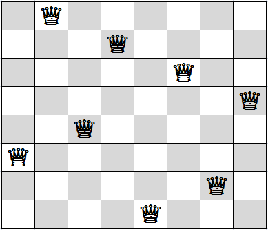
8 Queens Problem 

The N-queens problem is an effort to find a placement of N queens on an N by N chess board so that no two queens attack each other

At an initial state some queens may be attacking each other (i.e no 2 queens are on the same row, column, and diagonal).

GOAL: To evolve such a state using GA to find a state in which no 2 queens are attacking each other.

 

 

Genetic Algorithm

GA is one of the most popular meta-heuristic algorithms, its represent the space solution by population of chromosome and each chromosome work as a solution for the problem.  

GA give the optimal solution depending on fitness function and also depending on the structure of algorithm. The algorithm repeats the crossover of chromosome and the mutation operations until reaching the optimal solution (stop condition). 

 Algorithm

Input: Initial random solutions. 

Output: All possible solutions for eight queens problem. 

Step1: Generate 100 random solutions. This was done by initializing 100 vectors (with length of 64), the values in each vector are either one for the queen or zero for the empty square. Thus each vector will have eight queens distributed randomly. This is the initial population for GA with size equal 100 chromosomes.  

Step2: Evaluate the fitness of each chromosome (solution).  

Step3: Rank the chromosomes depending on their fitness’s values (small fitness values first).  

Step4: The 50 solutions that have the best fitness values are selected as parents and retained for the next generation. Those parents are then used to create another 50 offspring using single point crossover.  

Step5: The new solutions are mutated. 

Step6: Repeat steps 2-5 until a new solution to the 8-queens problem is found.